Linear mixed fluid-structure interaction system

This tutorial demonstrates the use of subdomain functionality and show how to describe a system consisting of multiple materials in Firedrake.

The tutorial was contributed by Tomasz Salwa and Onno Bokhove.

The model considered consists of fluid with a free surface and an elastic solid. We will be using interchangeably notions of fluid/water and structure/solid/beam. For simplicity (and speed of computation) we consider a model in 2D, however it can be easily generalised to 3D. The starting point is the linearised version (domain is fixed) of the fully nonlinear variational principle. In non-dimensional units:

\[\begin{split}0 = & \delta \int_0^{t_{\text{end}}} \int \left( \partial_t{\eta} \phi - \frac{1}{2} \eta^2 \right) {\mathrm d} S_f - \int \frac{1}{2} |\nabla \phi|^2 {\mathrm d} x_F \\ & + \int {\bf n} \cdot \partial_t {\bf X} \phi \, {\mathrm d} s_s\\ & + \int \rho_0 \partial_t {\bf X} \cdot {\bf U} - \frac 12 \rho_0 |{\bf U}|^2 - \frac 12 \lambda e_{ii}e_{jj} - \mu e_{ij} e_{ij}\, {\mathrm d} x_S \, {\mathrm d} t \, ,\end{split}\]

in which the first line contains integration over fluid domain, second, fluid-structure interface, and third, structure domain. The following notions are used:

• \(\eta\) - free surface deviation

• \(\phi\) - fluid flow potential

• \(\rho_0\) - structure density (in fluid density units)

• \(\lambda\) - first Lame constant (material parameter)

• \(\mu\) - second Lame constant (material parameter)

• \({\bf X}\) - structure displacement

• \({\bf U}\) - structure velocity

• \(e_{ij} = \frac{1}{2} \bigl( \frac{\partial X_j }{ \partial x_i } + \frac{ \partial X_i }{ \partial x_j } \bigr)\) - linear strain tensor; \(i\), \(j\) denote vector components

• \({\mathrm d} S_f\) - integration element over fluid free surface

• \({\mathrm d} s_s\) - integration element over structure-fluid interface

• \({\mathrm d} x_F\) - integration element over fluid domain

• \({\mathrm d} x_S\) - integration element over structure domain

After numerous manipulations (described in detail in [SBK17]) and evaluation of individual variations, the time-discrete equations, with symplectic Euler scheme, that we would like to implement in Firedrake, are:

\[\begin{split}\begin{aligned} \int v \phi^{n+1} \, {\mathrm d} S_f &= \int v (\phi^n - \Delta t \eta^n) \, {\mathrm d} S_f \\\\ % \int \rho_0 {\bf v} \cdot {\bf U}^{n+1} \, {\mathrm d} x_S\ \underline{+ \int {\bf n} \cdot {\bf v} \, \phi^{n+1} \, {\mathrm d} s_s} &= \rho_0 \int {\bf v} \cdot {\bf U}^n \, {\mathrm d} x_S \nonumber\\ &\hspace{4em}- \Delta t \int \left( \lambda \nabla \cdot {\bf v} \nabla \cdot {\bf X}^n + \mu \frac{\partial X^n_j}{\partial x_i} \left( \frac{\partial v_i}{\partial x_j} + \frac{\partial v_j}{\partial x_i} \right) \right) \, {\mathrm d} x_S \\ &\hspace{8em}\underline{ + \int {\bf n} \cdot {\bf v} \, \phi^n \, {\mathrm d} s_s }\\\\ % \int \nabla v \cdot \nabla \phi^{n+1} \, {\mathrm d} x_F\ \underline{- \int v {\bf n} \cdot {\bf U}^{n+1} \, {\mathrm d} s_s } &= 0 \\\\ %\hspace{1cm} (+ \text{Dirichlet BC at } \partial \Omega_f)\\ % \int v \eta^{n+1} \, {\mathrm d} S_f &= \int v \eta^n \, {\mathrm d} S_f + \Delta t \int \nabla v \cdot \nabla \phi^{n+1} \, {\mathrm d} x_F\\ &\hspace{4em}\underline{- \Delta t \int v {\bf n} \cdot {\bf U}^{n+1}\, {\mathrm d} s_s }\\\\ % \int {\bf v} \cdot {\bf X}^{n+1} \, {\mathrm d} x_S &= \int {\bf v} \cdot ( {\bf X}^n + \Delta t {\bf U}^{n+1} ) \, {\mathrm d} x_S \, . \end{aligned}\end{split}\]

The underlined terms are the coupling terms. Note that the first equation for \(\phi\) at the free surface is solved on the free surface only, the last equation for \({\bf X}\) in the structure domain, while the others are solved in both domains. Moreover, the second and third equations for \(\phi\) and \({\bf U}\) need to be solved simultaneously. The geometry of the system with initial condition is shown below.

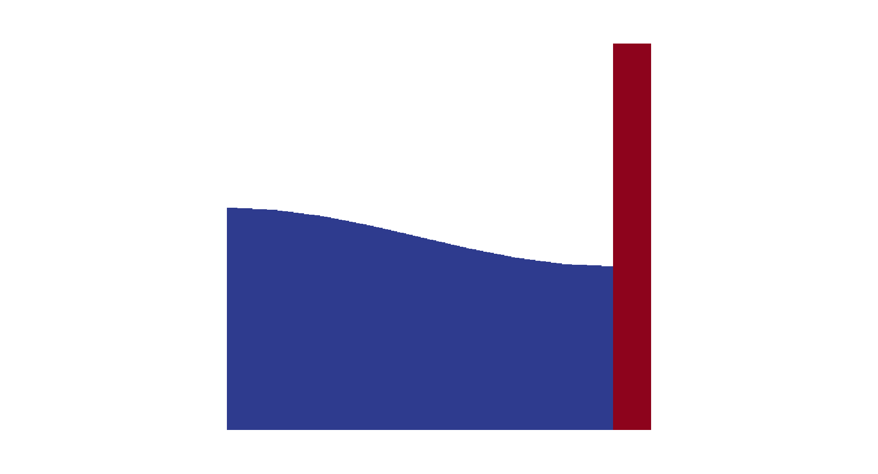
Geometry and initial condition in the system. Fluid (blue) with deflected free surface and the structure (red).

Now we present the code used to solve the system of equations above. We start with appropriate imports:

from firedrake import *
from firedrake.output import VTKFile
import math
import numpy as np

Then, we set parameters of the simulation:

# parameters in SI units
t_end = 5.0  # time of simulation [s]
dt = 0.005  # time step [s]
g = 9.8  # gravitational acceleration
# water
Lx = 20.0  # length of the tank [m] in x-direction; needed for computing initial condition
Lz = 10.0  # height of the tank [m]; needed for computing initial condition
rho = 1000.0  # fluid density in kg/m^2 in 2D [water]
# solid parameters
#  - we use a sufficiently soft material to be able to see noticeable structural displacement
rho_B = 7700.0  # structure density in kg/m^2 in 2D
lam = 1e7  # N/m in 2D - first Lame constant
mu = 1e7  # N/m in 2D - second Lame constant
# mesh
mesh = Mesh("L_domain.msh")
# these numbers must match the ones defined in the mesh file
fluid_id = 1  # fluid subdomain
structure_id = 2  # structure subdomain
bottom_id = 1  # structure bottom
top_id = 6  # fluid surface
interface_id = 9  # fluid-structure interface
# control parameters
output_data_every_x_time_steps = 20  # to avoid saving data every time step
coupling = True  # turn on coupling terms

The equations are in nondimensional units, hence we transform:

L = Lz
T = L / math.sqrt(g * L)
t_end /= T
dt /= T
Lx /= L
Lz /= L
rho_B /= rho
lam /= g * rho * L
mu /= g * rho * L
rho = 1.0  # or equivalently rho /= rho

Let us define function spaces, including the mixed one:

V_W = FunctionSpace(mesh, "CG", 1)
V_B = VectorFunctionSpace(mesh, "CG", 1)
mixed_V = V_W * V_B

Then, we define functions. First, in the fluid domain:

phi = Function(V_W, name="phi")
phi_f = Function(V_W, name="phi_f")  # at the free surface
eta = Function(V_W, name="eta")
trial_W = TrialFunction(V_W)
v_W = TestFunction(V_W)

Second, in the beam domain:

X = Function(V_B, name="X")
U = Function(V_B, name="U")
trial_B = TrialFunction(V_B)
v_B = TestFunction(V_B)

And last, mixed functions in the mixed domain:

trial_f, trial_s = TrialFunctions(mixed_V)
v_f, v_s = TestFunctions(mixed_V)
tmp_f = Function(V_W)
tmp_s = Function(V_B)
result_mixed = Function(mixed_V)

We need auxiliary indicator functions, that are 0 in one subdomain and 1 in the other. They are needed both in “CG” and “DG” space. We use the fact that the fluid and structure subdomains are defined in the mesh file with an appropriate ID number that Firedrake is able to recognise. That can be used in constructing indicator functions:

V_DG0_W = FunctionSpace(mesh, "DG", 0)
V_DG0_B = FunctionSpace(mesh, "DG", 0)

# Heaviside step function in fluid
I_W = Function(V_DG0_W)
par_loop(("{[i] : 0 <= i < f.dofs}", "f[i, 0] = 1.0"),
         dx(fluid_id),
         {"f": (I_W, WRITE)})
I_cg_W = Function(V_W)
par_loop(("{[i] : 0 <= i < A.dofs}", "A[i, 0] = fmax(A[i, 0], B[0, 0])"),
         dx,
         {"A": (I_cg_W, RW), "B": (I_W, READ)})

# Heaviside step function in solid
I_B = Function(V_DG0_B)
par_loop(("{[i] : 0 <= i < f.dofs}", "f[i, 0] = 1.0"),
         dx(structure_id),
         {"f": (I_B, WRITE)})
I_cg_B = Function(V_B)
par_loop(("{[i, j] : 0 <= i < A.dofs and 0 <= j < 2}", "A[i, j] = fmax(A[i, j], B[0, 0])"),
         dx,
         {"A": (I_cg_B, RW), "B": (I_B, READ)})

We use indicator functions to construct normal unit vector outward to the fluid domain at the fluid-structure interface:

n_vec = FacetNormal(mesh)
n_int = I_B("+") * n_vec("+") + I_B("-") * n_vec("-")

Now we can construct special boundary conditions that limit the solvers only to the appropriate subdomains of our interest:

class MyBC(DirichletBC):
    def __init__(self, V, value, markers):
        # Call superclass init
        # We provide a dummy subdomain id.
        super(MyBC, self).__init__(V, value, 0)
        # Override the "nodes" property which says where the boundary
        # condition is to be applied.
        self.nodes = np.unique(np.where(markers.dat.data_ro_with_halos == 0)[0])


def surface_BC():
    # This will set nodes on the top boundary to 1.
    bc = DirichletBC(V_W, 1, top_id)
    # We will use this function to determine the new BC nodes (all those
    # that aren't on the boundary)
    f = Function(V_W, dtype=np.int32)
    # f is now 0 everywhere, except on the boundary
    bc.apply(f)
    # Now I can use MyBC to create a "boundary condition" to zero out all
    # the nodes that are *not* on the top boundary:
    return MyBC(V_W, 0, f)


# same as above, but in the mixed space
def surface_BC_mixed():
    bc_mixed = DirichletBC(mixed_V.sub(0), 1, top_id)
    f_mixed = Function(mixed_V.sub(0), dtype=np.int32)
    bc_mixed.apply(f_mixed)
    return MyBC(mixed_V.sub(0), 0, f_mixed)


BC_exclude_beyond_surface = surface_BC()
BC_exclude_beyond_surface_mixed = surface_BC_mixed()
BC_exclude_beyond_solid = MyBC(V_B, 0, I_cg_B)
BC_exclude_beyond_water_mixed = MyBC(mixed_V.sub(0), 0, I_cg_W)
BC_exclude_beyond_solid_mixed = MyBC(mixed_V.sub(1), 0, I_cg_B)

Finally, we are ready to define the solvers of our equations. First, equation for \(\phi\) at the free surface:

a_phi_f = trial_W * v_W * ds(top_id)
L_phi_f = (phi_f - dt * eta) * v_W * ds(top_id)
LVP_phi_f = LinearVariationalProblem(a_phi_f, L_phi_f, phi_f, bcs=BC_exclude_beyond_surface)
LVS_phi_f = LinearVariationalSolver(LVP_phi_f)

Second, equation for the beam displacement \({\bf X}\), where we also fix it to the bottom by applying zero Dirichlet boundary condition:

a_X = dot(trial_B, v_B) * dx(structure_id)
L_X = dot((X + dt * U), v_B) * dx(structure_id)
# no-motion beam bottom boundary condition
BC_bottom = DirichletBC(V_B, as_vector([0.0, 0.0]), bottom_id)
LVP_X = LinearVariationalProblem(a_X, L_X, X, bcs=[BC_bottom, BC_exclude_beyond_solid])
LVS_X = LinearVariationalSolver(LVP_X)

Finally, we define solvers for \(\phi\), \({\bf U}\) and \(\eta\) in the mixed domain. In particular, value of \(\phi\) at the free surface is used as a boundary condition. Note that avg(…) is necessary for terms in expressions containing n_int, which is built in “DG” space:

# phi-U
# no-motion beam bottom boundary condition in the mixed space
BC_bottom_mixed = DirichletBC(mixed_V.sub(1), as_vector([0.0, 0.0]), bottom_id)
# boundary condition to set phi_f at the free surface
BC_phi_f = DirichletBC(mixed_V.sub(0), phi_f, top_id)
delX = nabla_grad(X)
delv_B = nabla_grad(v_s)
T_x_dv = lam * div(X) * div(v_s) + mu * (inner(delX, delv_B + transpose(delv_B)))
a_U = rho_B * dot(trial_s, v_s) * dx(structure_id)
L_U = (rho_B * dot(U, v_s) - dt * T_x_dv) * dx(structure_id)
a_phi = dot(grad(trial_f), grad(v_f)) * dx(fluid_id)
if coupling:
    a_U += dot(avg(v_s), n_int) * avg(trial_f) * dS  # avg(...) necessary here and below
    L_U += dot(avg(v_s), n_int) * avg(phi) * dS
    a_phi += -dot(n_int, avg(trial_s)) * avg(v_f) * dS
LVP_U_phi = LinearVariationalProblem(a_U + a_phi, L_U, result_mixed,
                                     bcs=[BC_phi_f,
                                          BC_bottom_mixed,
                                          BC_exclude_beyond_solid_mixed,
                                          BC_exclude_beyond_water_mixed])
LVS_U_phi = LinearVariationalSolver(LVP_U_phi)

# eta
a_eta = trial_W * v_W * ds(top_id)
L_eta = eta * v_W * ds(top_id) + dt * dot(grad(v_W), grad(phi)) * dx(fluid_id)
if coupling:
    L_eta += -dt * dot(n_int, avg(U)) * avg(v_W) * dS
LVP_eta = LinearVariationalProblem(a_eta, L_eta, eta, bcs=BC_exclude_beyond_surface)
LVS_eta = LinearVariationalSolver(LVP_eta)

Let us set the initial condition. We choose no motion at the beginning in both fluid and structure, zero displacement in the structure and deflected free surface in the fluid. The shape of the deflection is computed from the analytical solution:

# initial condition in fluid based on analytical solution
# compute analytical initial phi and eta
n_mode = 1
a = 0.0 * T / L ** 2  # in nondim units
b = 5.0 * T / L ** 2  # in nondim units
lambda_x = np.pi * n_mode / Lx
omega = np.sqrt(lambda_x * np.tanh(lambda_x * Lz))
x = mesh.coordinates
phi_exact_expr = a * cos(lambda_x * x[0]) * cosh(lambda_x * x[1])
eta_exact_expr = -omega * b * cos(lambda_x * x[0]) * cosh(lambda_x * Lz)

bc_top = DirichletBC(V_W, 0, top_id)
eta.assign(0.0)
phi.assign(0.0)
eta_exact = Function(V_W)
eta_exact.interpolate(eta_exact_expr)
eta.assign(eta_exact, bc_top.node_set)
phi.interpolate(phi_exact_expr)
phi_f.assign(phi, bc_top.node_set)

A file to store data for visualization:

outfile_phi = VTKFile("results_pvd/phi.pvd")

To save data for visualization, we change the position of the nodes in the mesh, so that they represent the computed dynamic position of the free surface and the structure:

def output_data():
    output_data.counter += 1
    if output_data.counter % output_data_every_x_time_steps != 0:
        return
    mesh_static = mesh.coordinates.vector().get_local()
    mesh.coordinates.vector().set_local(mesh_static + X.vector().get_local())
    mesh.coordinates.dat.data[:, 1] += eta.dat.data_ro
    outfile_phi.write(phi)
    mesh.coordinates.vector().set_local(mesh_static)


output_data.counter = -1  # -1 to exclude counting print of initial state

In the end, we proceed with the actual computation loop:

t = 0.0
output_data()

while t <= t_end + dt:
    t += dt
    print("time = ", t * T)
    # symplectic Euler scheme
    LVS_phi_f.solve()
    LVS_U_phi.solve()
    tmp_f, tmp_s = result_mixed.subfunctions
    phi.assign(tmp_f)
    U.assign(tmp_s)
    LVS_eta.solve()
    LVS_X.solve()

    output_data()

The result of the computation, visualised with paraview, is shown below.

The mesh is deflected for visualization only. As the model is linear, the actual mesh used for computation is fixed. Colours indicate values of the flow potential \(\phi\).

A python script version of this demo can be found here.

The mesh file is here. It can be generated with gmsh from this file with a command: gmsh -2 L_domain.geo.

An extended 3D version of this code is published here.

The work is based on the articles [SBK17] and [SBK16]. The authors gratefully acknowledge funding from European Commission, Marie Curie Actions - Initial Training Networks (ITN), project number 607596.

References

[SBK16]

Tomasz Salwa, Onno Bokhove, and Mark A. Kelmanson. Variational modelling of wave-structure interactions for offshore wind turbines. Extended paper for Int. Conf. on Ocean, Offshore and Arctic Eng., OMAE2016, Busan, South-Korea, June 2016. URL: https://asmedigitalcollection.asme.org/OMAE/proceedings-abstract/OMAE2016/49972/281268.

[SBK17] (1,2)

Tomasz Salwa, Onno Bokhove, and Mark A. Kelmanson. Variational modelling of wave–structure interactions with an offshore wind-turbine mast. Journal of Engineering Mathematics, Sep 2017. doi:10.1007/s10665-017-9936-4.