
Wind-Driven Gyres: Quasi-Geostrophic Limit
Contributed by Christine Kaufhold and Francis Poulin.
Building on the previous two demos that used the Quasi-Geostrophic (QG) model for the time-stepping and eigenvalue problem, we now consider how to determine a wind-driven gyre solution that includes bottom drag and nonlinear advection. This is referred to as the Nonlinear Stommel Problem.
This is a classical problem going back to [Sto48]. Even though it is far too simple to describe the dynamics of the real oceans quantitatively, it does explain qualitatively why we have western intensification in the world’s gyres. The curl of the wind stress adds vorticity into the gyres and the latitudinal variation in the Coriolis parameter causes a weak equatorward flow away from the boundaries (Sverdrup flow). It is because of the dissipation that arises near the boundaries that we must have western intensification. This was first shown by [Sto48] using simple bottom drag but it was only years later after [Mun50] did a similar calculation using lateral viscosity that people took the idea seriously.
After three quarters of a century we are still unable to parametrise the dissipative effects of the small scales so it is very difficult to get a good quantitative predictions as to the mean structure of the gyre that is generated. However, this demo aims to compute the structure of the oceanic gyre given particular parameters. The interested reader can read more about this in [Ped92] and [Val06]. In this tutorial we will consider the nonlinear Stommel problem.
Governing PDE: Stommel Problem
The nonlinear, one-layer, QG model equation that is driven by the winds above (say \(Q_{\textrm{winds}})\), which is the vorticity of the winds that drive the ocean from above) is,
with the Potential Vorticity (PV) and geostrophic velocities defined as
where \(\psi\) is the stream-function, \(\vec{u}=(u, v)\) is the velocity field, \(q\) is the PV, \(\beta\) is the latitudinal gradient of Coriolis parameter, and \(F\) is the rotational Froude number.
The non-conservative aspects of this model occur because of \(r\), the strength of the bottom drag, and \(Q_{\textrm{winds}}\), the vorticity of the winds. We pick the wind forcing as to generate a single gyre,
where \(L_y\) is the length of our domain and \(\tau\) is the strength of our wind forcing. By putting a \(2\) in front of the \(\pi\) we get a double gyre [Val06].
If we only look for steady solutions in time, we can ignore the time derivative term, and we get
We can write this out in one equation, which is the nonlinear Stommel problem:
Note that we dropped the \(-F \psi\) term in the nonlinear advection because the streamfunction does not change following the flow, and therefore, we can neglect that term entirely.
Weak Formulation
To build the weak form of the problem in Firedrake we must find the weak form of this equation. We begin by multiplying this equation by a test function, \(\phi\), which is in the same space as the streamfunction, and then integrate over the domain \(\Omega\),
The nonlinear term can be rewritten using the fact that the velocity is divergent free and then integrating by parts,
Note that because we have no normal flow boundary conditions the boundary contribution is zero. For the term with bottom drag we integrate by parts and use the fact that the streamfunction is zero on the walls
The boundary integral above vanishes because we are setting the streamfunction to be zero on the boundary.
Finally we can put the equation back together again to produce the weak form of our problem.
The above problem is the weak form of the nonlinear Stommel problem. The linear term arises from neglecting the nonlinear advection, and can easily be obtained by neglecting the first term on the left hand side.
Defining the Problem
Now that we know the weak form we are now ready to solve this using Firedrake!
First, we import the Firedrake, PETSc, NumPy and UFL packages,
from firedrake import *
from firedrake.petsc import PETSc
import numpy as np
import ufl
Next, we can define the geometry of our domain. In this example, we will be using a square of length one with 50 cells.
n0 = 50           # Spatial resolution
Ly = 1.0          # Meridonal length
Lx = 1.0          # Zonal length
mesh = RectangleMesh(n0, n0, Lx, Ly, reorder = None)
We can then define the Function Space within which the solution of the streamfunction will reside.
Vcg = FunctionSpace(mesh, 'CG', 3) # CG elements for Streamfunction
We will also impose no-normal flow strongly to ensure that the boundary condition \(\psi = 0\) will be met,
bc = DirichletBC(Vcg, 0.0, 'on_boundary')
Now we will define all the parameters we are using in this tutorial.
beta = Constant('1.0')      # Beta parameter
F = Constant('1.0')         # Burger number
r = Constant('0.2')         # Bottom drag
tau = Constant('0.001')     # Wind Forcing
x = SpatialCoordinate(mesh)
Qwinds = Function(Vcg).interpolate(-tau * cos(pi * (x[1]/Ly - 0.5)))
We can now define the Test Function and the Trial Function of this problem, both must be in the same function space:
phi, psi = TestFunction(Vcg), TrialFunction(Vcg)
We must define functions that will store our linear and nonlinear solutions. In order to solve the nonlinear problem, we use the linear solution as a guess for the nonlinear problem.
psi_lin = Function(Vcg, name='Linear Streamfunction')
psi_non = Function(Vcg, name='Nonlinear Streamfunction')
We can finally write down the linear Stommel equation in its weak form. We will use the solution to this as the input for the nonlinear Stommel equation.
a = - r * inner(grad(psi), grad(phi)) * dx - F * psi * phi * dx + beta * psi.dx(0) * phi * dx
L = Qwinds * phi * dx
We set-up an elliptic solver for this problem, and solve for the linear streamfunction,
linear_problem = LinearVariationalProblem(a, L, psi_lin, bcs=bc)
linear_solver = LinearVariationalSolver(linear_problem,
                                        solver_parameters= {'ksp_type': 'preonly',
                                                            'pc_type': 'lu'})
linear_solver.solve()
We will employ the solution to the linear problem as the initial guess for the nonlinear one:
psi_non.assign(psi_lin)
And now we can define the weak form of the nonlinear problem. Note that the problem is stated in residual form so there is no trial function.
G = - inner(grad(phi), perp(grad(psi_non))) * div(grad(psi_non)) * dx \
    -r * inner(grad(psi_non), grad(phi)) * dx - F * psi_non * phi * dx \
    + beta * psi_non.dx(0) * phi * dx \
    - Qwinds * phi * dx
We solve for the nonlinear streamfunction now by setting up another elliptic solver,
nonlinear_problem = NonlinearVariationalProblem(G, psi_non, bcs=bc)
nonlinear_solver = NonlinearVariationalSolver(nonlinear_problem,
                                              solver_parameters= {'snes_type': 'newtonls',
                                                                  'ksp_type': 'preonly',
                                                                  'pc_type': 'lu'})
nonlinear_solver.solve()
Now that we have the full solution to the nonlinear Stommel problem,
we can plot it using the tripcolor function
try:
    import matplotlib.pyplot as plt
except:
    warning("Matplotlib not imported")

try:
    from firedrake.pyplot import tripcolor
    fig, axes = plt.subplots()
    colors = tripcolor(psi_non, axes=axes)
    fig.colorbar(colors)
except Exception as e:
    warning("Cannot plot figure. Error msg '%s'" % e)

try:
    plt.show()
except Exception as e:
    warning("Cannot show figure. Error msg '%s'" % e)

file = VTKFile('Nonlinear Streamfunction.pvd')
file.write(psi_non)
We can also see the difference between the linear solution and the nonlinear solution. We do this by defining a weak form. (Note: other approaches may be possible.)
tf, difference = TestFunction(Vcg), TrialFunction(Vcg)

difference = assemble(psi_lin - psi_non)

try:
    fig, axes = plt.subplots()
    colors = tripcolor(difference, axes=axes)
    fig.colorbar(colors)
except Exception as e:
    warning("Cannot plot figure. Error msg '%s'" % e)

try:
    plt.show()
except Exception as e:
    warning("Cannot show figure. Error msg '%s'" % e)

file = VTKFile('Difference between Linear and Nonlinear Streamfunction.pvd')
file.write(difference)
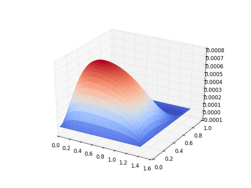
Below is a plot of the linear solution to the QG wind-driven Stommel gyre.
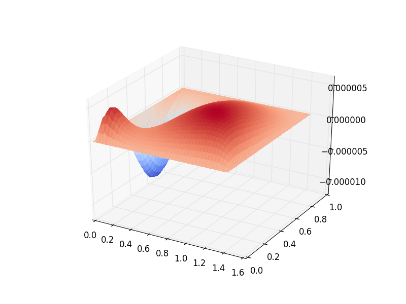
Below is a plot of the difference between the linear and nonlinear solutions to the QG wind-driven Stommel gyre.
This demo can be found as a Python script in qg_winddrivengyre.py.
References
Walter H. Munk. On the wind-driven ocean circulation. Journal of Meteorology, 7:79–93, 1950. doi:10.1175/1520-0469(1950)007<0080:OTWDOC>2.0.CO;2.
Joseph Pedlosky. Geophysical Fluid Dynamics. Springer study edition. Springer New York, 1992. ISBN 9780387963877.
Henry Stommel. The westward intensifciation of wind driven ocean currents. Trans. Am. Geophys. Union, 29:202–206, 1948. doi:10.1007/s10915-004-4635-5.