Interfacing directly with PETSc ¶

Introduction ¶

Sometimes, the system we wish to solve can not be described purely in terms of a sum of weak forms that we can then assemble. Or else, it might be, but the resulting assembled operator would be dense. In this chapter, we will see how to solve such problems in a “matrix-free” manner, using Firedrake to assemble the pieces and then providing a matrix object to PETSc which is unassembled. Note that this is a lower-level interface than that described in Matrix-free operators, so you should try that first to see if it suits your needs.

To take a concrete example, let us consider a linear system obtained from a normal variational problem, augmented with a rank-1 perturbation:

\[B := A + \vec{u} \vec{v}^T.\]

Such operators appear, for example, in limited memory quasi-Newton methods such as L-BFGS or Broyden.

The matrix \(B\) is dense, however its action on a vector may be computed in only marginally more work than computing the action of \(A\) since

\[B \vec{x} \equiv A \vec{x} + \vec{u} (\vec{v} \cdot \vec{x}).\]

Accessing PETSc objects ¶

Firedrake builds on top of PETSc for its linear algebra, and therefore all assembled forms provide access to the underlying PETSc object. For assembled bilinear forms, the PETSc object is a Mat; for assembled linear forms, it is a Vec. The ways we access these are different. For a bilinear form, the matrix is obtained with:

petsc_mat = assemble(bilinear_form).M.handle

For a linear form, we need to use a context manager. There are two options available here, depending on whether we want read-only or read-write access to the PETSc object. For read-only access, we use:

with assemble(linear_form).dat.vec_ro as v:
    petsc_vec_ro = v

For write-only access, use .vec_wo, and for read-write access, use:

with assemble(linear_form).dat.vec as v:
    petsc_vec = v

These context managers ensure that if PETSc writes to the vector, Firedrake sees the modification of the values.

Plotting the sparsity of a PETSc `Mat`¶

Given a PETSc matrix of type 'seqaij', we may access its compressed sparse row format and convert to that used in SciPy in the following way:

import scipy.sparse as sp

indptr, indices, data = petsc_mat.getValuesCSR()
scipy_mat = sp.csr_matrix((data, indices, indptr), shape=petsc_mat.getSize())

The sparsity pattern may then be straightforwardly plotted using matplotlib:

import matplotlib.pyplot as plt

plt.spy(scipy_mat)

Building an operator ¶

To solve the linear system \(Bx = b\) we need to define the operator \(B\) such that PETSc can use it. To do this, we build a Python class that provides a mult method:

class MatrixFreeB(object):

    def __init__(self, A, u, v):
        self.A = A
        self.u = u
        self.v = v

    def mult(self, mat, x, y):
        # y <- A x
        self.A.mult(x, y)

        # alpha <- v^T x
        alpha = self.v.dot(x)

        # y <- y + alpha*u
        y.axpy(alpha, self.u)

Now we must build a PETSc Mat and indicate that it should use this newly defined class to compute the matrix action:

# Import petsc4py namespace
from firedrake.petsc import PETSc

B = PETSc.Mat().create()

# Assemble the bilinear form that defines A and get the concrete
# PETSc matrix
A = assemble(bilinear_form).M.handle

# Now do the same for the linear forms for u and v, making a copy

with assemble(u_form).dat.vec_ro as u_vec:
    u = u_vec.copy()

with assemble(v_form).dat.vec_ro as v_vec:
    v = v_vec.copy()


# Build the matrix "context"
Bctx = MatrixFreeB(A, u, v)

# Set up B
# B is the same size as A
B.setSizes(A.getSizes())

B.setType(B.Type.PYTHON)
B.setPythonContext(Bctx)
B.setUp()

The next step is to build a linear solver object to solve the system. For this we need a PETSc KSP:

ksp = PETSc.KSP().create()

ksp.setOperators(B)

ksp.setFromOptions()

Now we can solve a system using this ksp object:

solution = Function(V)

rhs = assemble(rhs_form)

with rhs.dat.vec_ro as b:
    with solution.dat.vec as x:
        ksp.solve(b, x)

Defining a preconditioner ¶

Note

In many cases it is not necessary to drop to this low a level to construct problem-specific preconditioners. More details on this approach are discussed in the manual section on Preconditioning infrastructure.

Since PETSc only knows how to compute the action of \(B\), and does not have access to any of the entries, it will not be able to build a preconditioner for the linear solver. To use a preconditioner, we have to provide PETSc with one. We can do this in one of two ways.

Provide an assembled matrix to the KSP object to be used as a preconditioning matrix. For example, we might use the matrix \(A\). In this case, we merely have to call ksp.setOperators with two arguments:
```
ksp.setOperators(B, A)
```
Now we solve the system \(Bx = b\), using \(A\) to build a preconditioner.
Provide our own PC object to be used as the preconditioner. This is somewhat more involved. As we did to define the matrix-free action of \(B\), we need to build an object that applies the action of our chosen preconditioner. If we know that our matrix \(B\) has some special structure, this can be more efficient than the previous method.

Providing a custom preconditioner ¶

Recall that we do not explicitly form \(B\) since it is dense, and subsequently its inverse is as well. However, since we know that \(B\) is formed of a full-rank invertible matrix, \(A\), plus a rank-1 update, it is possible to compute its inverse reasonably cheaply using the Sherman-Morrison formula. Let \(A\) be invertible and \(u\) and \(v\) be column vectors such that \(1 + v^T A^{-1} u \neq 0\) then:

\[B^{-1} = (A + u v^T)^{-1} = A^{-1} - \frac{A^{-1}u v^T A^{-1}}{1 + v^T A^{-1} u}.\]

Hence, we see that we can apply the action of \(B^{-1}\) on a vector using only the action of \(A^{-1}\) and some dot products.

With these mathematical preliminaries out of the way, let us move on to the implementation. We need to define an object which has an apply method which applies the action of our preconditioner to a vector. The PETSc PC object will be created with access to the operators we have provided to our solver, so for this class, we won’t pass \(A\), \(u\) and \(v\) explicitly, but rather extract them from the operators in a setUp method:

class MatrixFreePC(object):

    def setUp(self, pc):
        B, P = pc.getOperators()
        # extract the MatrixFreeB object from B
        ctx = B.getPythonContext()
        self.A = ctx.A
        self.u = ctx.u
        self.v = ctx.v
        # Here we build the PC object that uses the concrete,
        # assembled matrix A.  We will use this to apply the action
        # of A^{-1}
        self.pc = PETSc.PC().create()
        self.pc.setOptionsPrefix("mf_")
        self.pc.setOperators(self.A)
        self.pc.setFromOptions()
        # Since u and v do not change, we can build the denominator
        # and the action of A^{-1} on u only once, in the setup
        # phase.
        tmp = self.A.createVecLeft()
        self.pc.apply(self.u, tmp)
        self._Ainvu = tmp
        self._denom = 1 + self.v.dot(self._Ainvu)

    def apply(self, pc, x, y):
        # y <- A^{-1}x
        self.pc.apply(x, y)
        # alpha <- (v^T A^{-1} x) / (1 + v^T A^{-1} u)
        alpha = self.v.dot(y) / self._denom
        # y <- y - alpha * A^{-1}u
        y.axpy(-alpha, self._Ainvu)

Now we extract the PC object from the KSP linear solver and indicate that it should use our matrix free preconditioner

ksp = PETSc.KSP().create()
ksp.setOperators(B)
ksp.setUp()
pc = ksp.pc
pc.setType(pc.Type.PYTHON)
pc.setPythonContext(MFPC())
ksp.setFromOptions()

before going on to solve the system as before:

solution = Function(V)

rhs = assemble(rhs_form)

with rhs.dat.vec_ro as b:
    with solution.dat.vec as x:
        ksp.solve(b, x)

Accessing the PETSc mesh representation ¶

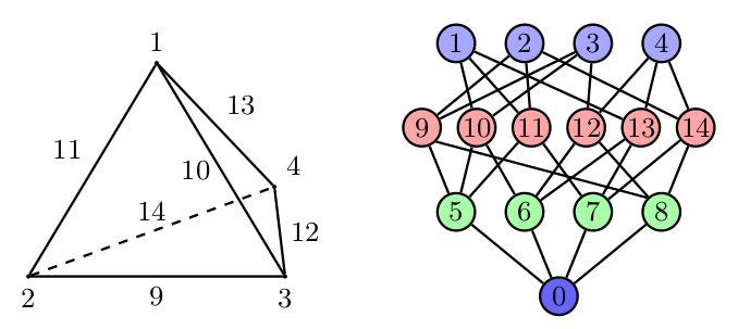
Under the hood, Firedrake uses PETSc’s DMPlex unstructured mesh representation. It uses a hierarchical approach, where entities of different dimension are put on different levels of the hierarchy. The single tetrahedral element shown on the left below may be interpreted using the graph representation on the right. Entities of dimension zero (vertices) are shown at the top. Entities of dimension one (edges) are shown on the next level down. Entities of dimension two (faces) are shown on the penultimate level and the (dimension three) element itself is on the bottom level. Edges in the graph indicate which entities own/are owned by others.

The DMPlex associated with a given mesh may be accessed via its topology_dm attribute:

plex = mesh.topology_dm

All entities in a DMPlex are given a unique number. The range of these numbers may be deduced using the method plex.getDepthStratum, whose only argument is the entity dimension sought. For example, 0 for vertices, 1 for edges, etc. Similarly, the method plex.getHeightStratum can be used for codimension access. For example, height 0 corresponds to cells. The hierarchical DMPlex structure may be traversed using other methods, such as plex.getCone, plex.getSupport and plex.getTransitiveClosure. See the Firedrake DMPlex paper and the PETSc manual for details.

If vertex coordinate information is to be accessed from the DMPlex then we must first establish a mapping between its numbering and the coordinates in the Firedrake mesh. This is done by establishing a ‘section’. A section provides a way of associating data with the mesh - in this case, coordinate field data. For a \(d\)-dimensional mesh, we seek to establish offsets to recover \(d\)-tuple coordinates for the degrees of freedom.

For a linear mesh, we seek \(d\) values at each vertex and no values for entities of higher dimension. In 2D, for example, this corresponds to the array

\[(d, 0, 0).\]

For an order \(p\) Lagrange mesh, it is a little more complicated. In the 2D triangular case, we require the following entities:

\[(d, d(p-1), d(p-1)(p-2)/2).\]

Accordingly, set

dim = mesh.topological_dimension()
gdim = mesh.geometrical_dimension()
entity_dofs = np.zeros(dim+1, dtype=np.int32)
entity_dofs[0] = gdim
entity_dofs[1] = gdim*(p-1)
entity_dofs[2] = gdim*((p-1)*(p-2))//2

We then use Firedrake’s helper function for creating a PETSc section to establish the mapping:

coord_section = mesh.create_section(entity_dofs)
plex = mesh.topology_dm
plex_coords = plex.getCoordinateDM()
plex_coords.setDefaultSection(coord_section)
coords_local = plex_coords.createLocalVec()
coords_local.array[:] = np.reshape(mesh.coordinates.dat.data_ro_with_halos, coords_local.array.shape)
plex.setCoordinatesLocal(coords_local)

We can then extract coordinates for node i belonging to entity d (according to the DMPlex numbering) by

dofs = coord_section.getDof(d)
offset = coord_section.getOffset(d)//dim + i
coord = mesh.coordinates.dat.data_ro_with_halos[offset]
print(f"Node {i} belonging to entity {d} has coordinates {coord}")