
Hamiltonian-structure-preserving implementation of the Benjamin-Bona-Mahoney equation
This demo solves the Benjamin-Bona-Mahony equation:
posed on a bounded interval with periodic boundaries.
BBM is known to have a Hamiltonian structure, and there are several canonical polynomial invariants:
The BBM invariants are the total momentum \(I_1\), the \(H^1\)-energy norm \(I_2\), and the Hamiltonian \(I_3\). The Hamiltonian variational formulation reads
For all test functions \(v, v_H\) in a suitable function space. The numerical scheme in this demo introduces the \(H^1\)-Riesz representative of the Fréchet derivative of the Hamiltonian \(\frac{\delta I_3}{\delta u}\) as the auxiliary variable \(\tilde{w}_H\).
Standard Gauss-Legendre and continuous Petrov-Galerkin (cPG) methods conserve the first two invariants exactly (up to roundoff and solver tolerances). They do quite well, but are inexact for the cubic one. Here, we consider the reformulation in Andrews and Farrell, “Enforcing conservation laws and dissipation inequalities numerically via auxiliary variables” (arXiv:2407.11904, to appear in SIAM J. Scientific Computing) that preserves the third invariant at the expense of the second. This method has an auxiliary variable in the system and requires a continuously differentiable spatial discretization (1D Hermite elements in this case). The time discretization puts the main unknown in a continuous space and the auxiliary variable in a discontinuous one. See equation (7.17) of Boris Andrews’ thesis for the particular formulation.
Firedrake, Irksome, and other imports:
from firedrake import (Constant, Function, FunctionSpace,
    PeriodicIntervalMesh, SpatialCoordinate, TestFunction, TrialFunction,
    assemble, derivative, dx, errornorm, exp, grad, inner,
    interpolate, norm, plot, project, replace, solve, split
)

from irksome import Dt, TimeStepper, ContinuousPetrovGalerkinScheme

import matplotlib.pyplot as plt
import numpy
Next, we define the domain and the exact solution
N = 8000
L = 100
h = L / N
msh = PeriodicIntervalMesh(N, L)
x, = SpatialCoordinate(msh)

t = Constant(0)
inv_dt = N // (10 * L)
tfinal = 18
Nt = tfinal * inv_dt
dt = Constant(tfinal / Nt)

c = Constant(0.5)
center = Constant(40.0)
delta = -c * center

def sech(x):
    return 2 / (exp(x) + exp(-x))

uexact = 3 * c**2 / (1-c**2) \
    * sech(0.5 * (c * x - c * t / (1 - c ** 2) + delta))**2
This sets up the function space for the unknown \(u\) and auxiliary variable \(\tilde{w}_H\):
space_deg = 3
time_deg = 1

V = FunctionSpace(msh, "Hermite", space_deg)
Z = V * V
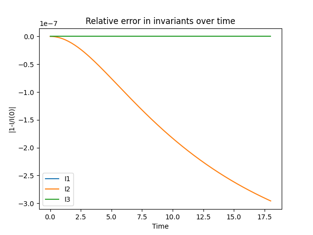
We next define the BBM invariants. Again, the discrete formulation preserves \(I_1\) and \(I_3\) up to solver tolerances and roundoff errors, but \(I_2\) is preserved up to a bounded oscillation
def h1inner(u, v):
    return inner(u, v) + inner(grad(u), grad(v))

def I1(u):
    return u * dx

def I2(u):
    return h1inner(u, u) * dx

def I3(u):
    return (u**2 / 2 + u**3 / 6) * dx
We project the initial condition on \(u\), but we also need a consistent initial condition for the auxiliary variable. We need to find \(\tilde{w}_H \in V\) such that
uwH = Function(Z)
u0, wH0 = uwH.subfunctions

v = TestFunction(V)
w = TrialFunction(V)
a = h1inner(w, v) * dx
dHdu = derivative(I3(u0), u0, v)

solve(a == h1inner(uexact, v)*dx, u0)
solve(a == dHdu, wH0)
Visualize the initial condition:
fig, axes = plt.subplots(1)
plot(Function(FunctionSpace(msh, "CG", 1)).interpolate(u0), axes=axes)
axes.set_title("Initial condition")
axes.set_xlabel("x")
axes.set_ylabel("u")
plt.savefig("bbm_init.png")

Set up the semidiscrete form as usual:
u, wH = split(uwH)
v, vH = split(TestFunction(Z))

F = h1inner(Dt(u) + wH.dx(0), v) * dx
F += h1inner(wH, vH) * dx - derivative(I3(u), u, vH)
Next, we set up the cPG scheme. We specify quadrature_degree=”auto” to override the default quadrature of degree 2*time_deg-1. This automatically estimates the quadrature degree for each individual term in F. The degree estimation algorithm will only be exact for polynomial nonlinearities, such as the cubic term in I3. For complicated nonlinearities, the estimated degree might be too large and result in very slow compilation and runtime. The quadrature degree might be optionally capped via max_quadrature_degree keyword argument.
scheme = ContinuousPetrovGalerkinScheme(time_deg, quadrature_degree="auto",
                                        max_quadrature_degree=3*time_deg-1)
This sets up the cPG time stepper. There are two fields in the unknown, we indicate that the second one is an auxiliary and hence to be discretized in the DG test space instead by passing the aux_indices keyword:
stepper = TimeStepper(F, scheme, t, dt, uwH, aux_indices=[1])
UFL expressions for the invariants, which we are going to track as we go through time steps:
times = [float(t)]
functionals = (I1(u), I2(u), I3(u))
invariants = [tuple(map(assemble, functionals))]
Do the time-stepping:
for _ in range(Nt):
    stepper.advance()

    invariants.append(tuple(map(assemble, functionals)))

    i1, i2, i3 = invariants[-1]
    t.assign(float(t) + float(dt))
    times.append(float(t))

    print(f'{float(t):.15f}, {i1:.15f}, {i2:.15f}, {i3:.15f}')
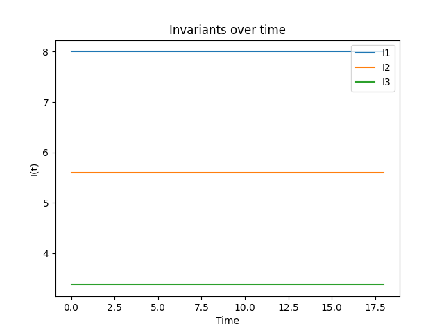
Visualize invariant preservation:
axes.clear()
invariants = numpy.array(invariants)

lbls = ("I1", "I2", "I3")

for i in (0, 1, 2):
    plt.plot(times, invariants[:, i], label=lbls[i])
axes.set_title("Invariants over time")
axes.set_xlabel("Time")
axes.set_ylabel("I(t)")
axes.legend()
plt.savefig("invariants.png")
axes.clear()

for i in (0, 1, 2):
    plt.plot(times, 1.0 - invariants[:, i]/invariants[0, i], label=lbls[i])
axes.set_title("Relative error in invariants over time")
axes.set_xlabel("Time")
axes.set_ylabel("|1-I/I(0)|")
axes.legend()
plt.savefig("invariant_errors.png")
Visualize the solution at final time step:
axes.clear()
plot(Function(FunctionSpace(msh, "CG", 1)).interpolate(u0), axes=axes)
axes.set_title(f"Solution at time {tfinal}")
axes.set_xlabel("x")
axes.set_ylabel("u")
plt.savefig("bbm_final.png")
