
Warning
You are reading a version of the website built against the unstable main branch. This content is liable to change without notice and may be inappropriate for your use case.
You can find the documentation for the current stable release here.
Creating Firedrake-compatible meshes in Gmsh
The purpose of this demo is to demonstrate methods available through Gmsh to create meshes compatible with Firedrake. It overviews the creation the same mesh, three different ways:
Constructing a GEO file
Using the Gmsh API
Using OpenCASCADE through Gmsh
For more details about Gmsh, please refer to the Gmsh documentation. The Gmsh syntax used in this document is for Gmsh version 4.4.1.
import matplotlib.pyplot as plt
from firedrake import *
import gmsh
As example, we will construct and mesh the following geometry: a rectangle with a disc in the middle. In the picture, numbers in black refer to Gmsh point tags, whereas numbers in red refer to Gmsh curve tags (see below).
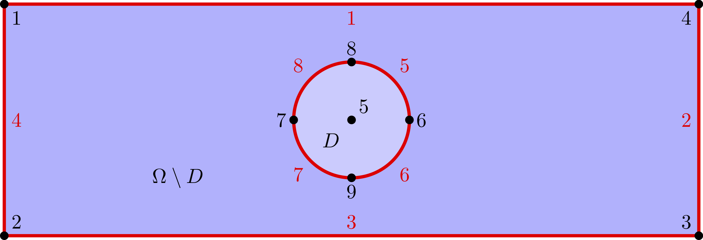
Relative to a central origin, (x0, y0, z0), the rectangle is parameterised by its length L,
and width, W. Likewise, the disc is parameterised its radius, R. The target element size is
set to dx_rec=0.5 and dx_disc=0.1 to generate finer triangles around the disc.
x0, y0, z0 = 0., 0., 0.
L = 12.
W = 4.
R = 1.
dx_rec  = 0.5
dx_disc = 0.1
Constructing a GEO file
The first thing we need to do is to create a Gmsh gmsh.geo,
which is the geometry recipe for Gmsh.
We begin by defining the four corners of a bounding rectangle. We specify the x,y, and z(=0) coordinates, as well as the target element size at these corners.
Point(1) = {-6,  2, 0, 0.5};
Point(2) = {-6, -2, 0, 0.5};
Point(3) = { 6, -2, 0, 0.5};
Point(4) = { 6,  2, 0, 0.5};
Note
Gmsh tracks most objects through a combination of its dimension, dim
and an integer tag, tag, which must be unique to the object. For example,
Point(1) has dimension 0 and a unique tag 1, while Line(1) has
dimension 1 and a unique tag 1.
Then, we define 5 points to describe a circle.
Point(5) = { 0,  0, 0, 0.1};
Point(6) = { 1,  0, 0, 0.1};
Point(7) = {-1,  0, 0, 0.1};
Point(8) = { 0,  1, 0, 0.1};
Point(9) = { 0, -1, 0, 0.1};
Then, we create 8 edges: 4 for the rectangle and 4 for the circle.
Note that the Gmsh command Circle requires the arc to be
strictly smaller than \(\pi\).
Line(1) = {1, 4};
Line(2) = {4, 3};
Line(3) = {3, 2};
Line(4) = {2, 1};
Circle(5) = {8, 5, 6};
Circle(6) = {6, 5, 9};
Circle(7) = {9, 5, 7};
Circle(8) = {7, 5, 8};
Then, we glue together the rectangle edges and, separately, the circle edges.
Note that Line, Circle, and Curve Loop (as well as Physical Curve below)
are all curves in Gmsh and must possess a unique tag.
Curve Loop( 9) = {1, 2, 3, 4};
Curve Loop(10) = {8, 5, 6, 7};
Then, we define two plane surfaces: the rectangle without the disc first, and the disc itself then.
Plane Surface(1) = {9, 10};
Plane Surface(2) = {10};
Finally, we group together some edges and define Physical entities.
Firedrake uses the tag of each physical entity to distinguish
between parts of the mesh (see the concrete example at the end of this page).
Physical Curve("HorEdges", 11) = {1, 3};
Physical Curve("VerEdges", 12) = {2, 4};
Physical Curve("Circle", 13) = {8, 7, 6, 5};
Physical Surface("PunchedDom", 3) = {1};
Physical Surface("Disc", 4) = {2};
For simplicity, we have gathered all this commands in the file immersed_domain.geo. To generate a mesh using this file, you can type the following command in the terminal
gmsh -2 immersed_domain.geo -format msh2
Note
The -2 flag indicates whether the mesh will be 2 or 3 dimensions. Depending on your
version of Gmsh and DMPlex, the Gmsh option -format msh2 may be omitted.
Using the Gmsh API
We can alternatively use python commands enabled through the Gmsh API to build, save, and read the mesh into Firedrake from within a python script. This allows for parameter flexibility and improved readability of the mesh generation code.
We first need to initialize the Gmsh API and create a new empty mesh model.
gmsh.initialize()
model = gmsh.model
model.add("gmsh_api_demo")
As before, we define the four rectangle corner points and target element size.
rectangle_points = [
model.geo.addPoint(x0 - L/2, y0 + W/2, z0, dx_rec, tag = 1), # top left
model.geo.addPoint(x0 - L/2, y0 - W/2, z0, dx_rec, tag = 2), # bottom left
model.geo.addPoint(x0 + L/2, y0 - W/2, z0, dx_rec, tag = 3), # bottom right
model.geo.addPoint(x0 + L/2, y0 + W/2, z0, dx_rec, tag = 4)  # top right
]
Then, we define 5 points to describe a circle.
center = model.geo.addPoint(x0, y0, z0, tag = 5)
circle_points = [
model.geo.addPoint(x0 - R, y0, z0, dx_disc, tag = 6),
model.geo.addPoint(x0, y0 + R, z0, dx_disc, tag = 7),
model.geo.addPoint(x0 + R, y0, z0, dx_disc, tag = 8),
model.geo.addPoint(x0, y0 - R, z0, dx_disc, tag = 9)
]
Then, we create 8 edges: 4 for the rectangle and 4 for the circle.
rectangle_lines = [
model.geo.addLine(rectangle_points[0], rectangle_points[1], tag = 1), # left
model.geo.addLine(rectangle_points[1], rectangle_points[2], tag = 2), # bottom
model.geo.addLine(rectangle_points[2], rectangle_points[3], tag = 3), # right
model.geo.addLine(rectangle_points[3], rectangle_points[0], tag = 4)  # top
]

circle_arcs =[
model.geo.addCircleArc(circle_points[0], center, circle_points[1], tag = 5),
model.geo.addCircleArc(circle_points[1], center, circle_points[2], tag = 6),
model.geo.addCircleArc(circle_points[2], center, circle_points[3], tag = 7),
model.geo.addCircleArc(circle_points[3], center, circle_points[0], tag = 8)
]
We then combine the edges into a closed loop for both the rectangle and
the circle used to define a surface for the area outside and inside the
inscribed circle, respectively. In the addPlaneSurface function by
convention, the first Curve Loop defines the outer boundary and
anything after in the list is treated as the boundary of a hole (or holes)
in the domain. These need to be registered to the model with synchronize
before we can use them.
rectangle_loop = model.geo.addCurveLoop(rectangle_lines, tag = 9)
circle_loop = model.geo.addCurveLoop(circle_arcs, tag = 10)

punched_surface = model.geo.addPlaneSurface([rectangle_loop,circle_loop], tag = 1)
circle_surface = model.geo.addPlaneSurface([circle_loop], tag = 2)
model.geo.synchronize()
Finally, we group together some edges and define Physical entities.
model.addPhysicalGroup(dim = 1, tags = [rectangle_lines[1], rectangle_lines[3]], tag = 11, name="HorEdges")
model.addPhysicalGroup(dim = 1, tags = [rectangle_lines[0], rectangle_lines[2]], tag = 12, name="VerEdges")
model.addPhysicalGroup(dim = 1, tags = circle_arcs, tag = 13, name="Circle")
model.addPhysicalGroup(dim = 2, tags = [punched_surface], tag = 3, name="PunchedDom")
model.addPhysicalGroup(dim = 2, tags = [circle_surface], tag = 4, name="Disc")
A number of meshing options are available. In particular, the algorithm for mesh generation and can be set globally or for individual surfaces.
2D: 1: MeshAdapt, 2: Automatic, 3: Initial mesh only, 5: Delaunay, 6: Frontal-Delaunay (default),7: BAMG, 8: Frontal-Delaunay for Quads, 9: Packing of Parallelograms, 11: Quasi-structured Quad
3D: Delaunay (default) 3: Initial mesh only 4: Frontal 7: MMG3D 9: R-tree 10: HXT
For more information see the Gmsh algorithm overview.
When writing the mesh to file, the format is determined by the file extension. For example,
.msh2 for Gmsh 2.x, .msh for GMSH 4.x.
gmsh.option.setNumber("Mesh.Algorithm", 6)
gmsh.option.setNumber("Mesh.MshFileVersion", 4.1)
gmsh.model.mesh.generate(2)
gmsh.write('gmsh_api_demo.msh')
We close the Gmsh API kernel after finalising the mesh.
gmsh.finalize()
Using OpenCASCADE through Gmsh
Using OpenCASCADE through Gmsh, we define higher level geometries such as rectangles and discs directly. It also has additional 3D capability, and integration not illustrated here. Please see the OpenCASCADE documentation in Gmsh for more details.
As with the Gmsh API, we initialize and start constructing a new mesh model.
gmsh.initialize()
model = gmsh.model
gmsh.model.add("gmsh_occ_demo")
We first use OpenCASCADE to create a rectangle and a cylinder object. This automates
the create of points, lines, and surfaces. Both objects need to be registered to the
model with synchronize before we can use them.
rectangle_obj_tag = model.occ.addRectangle(x0 - L/2, y0 - W/2, z0, L, W, tag = 1)
disc_obj_tag = model.occ.addDisk(x0, y0, z0, rx = R, ry = R, tag = 2)
model.occ.synchronize()
To create the whole, we use the method occ.cut with the option removeTool=False to
retain the disc interior (which would be otherwise deleted by default). The occ.cut method
takes and returns a list of tuples (dimension, tag) as do other functions such as
getBoundary used below. We save the tag of the combined object for later use
and register the new object to the model with synchronize.
punched_surface = model.occ.cut([(2, rectangle_obj_tag)], [(2, disc_obj_tag)], removeTool=False)
punched_surface_tag = punched_surface[0][0][1]
model.occ.synchronize()
We then extract the boundary from the objects. We extract the the punched surface
lines along with disc points to define the Physical groups. It returns boundaries
per entity (combined = false) or as a single shape (combined = true), and
adjust the signs to reflect orientation if oriented = true. The boundary operator
is applied down to point-level, or dimension 0, when recursive = True.
punched_lines = model.getBoundary([(2, punched_surface_tag)],
                                     combined = True, oriented = True, recursive = False)
disc_points = model.getBoundary([(2, disc_obj_tag)],
                                     combined = True, oriented = True, recursive = True)
We set the mesh resolution using setSize. The choice here is to first set all the
zero-dimensional points to the background size, and then override the mesh size for the
points on the circle boundary. Another strategy documented in the Gmsh manual is to
identify the desired points by a bounding box search.
model.mesh.setSize(gmsh.model.occ.getEntities(0), dx_rec)
model.mesh.setSize(disc_points, dx_disc)
We parse just the line tags to create a list of physical group tags. In this case the assignment of the lines was done manually through trial and inspection. TODO: add a function to automatically assign the lines to the physical groups.
punched_line_tags = [abs(line) for dim,line in punched_lines]
model.addPhysicalGroup(dim = 1, tags = [punched_line_tags[1], punched_line_tags[4]], tag = 11, name="HorEdges")
model.addPhysicalGroup(dim = 1, tags = [punched_line_tags[2], punched_line_tags[3]], tag = 12, name="VertEdges")
model.addPhysicalGroup(dim = 1, tags = [punched_line_tags[0]], tag = 13, name="CircleEdge")
model.addPhysicalGroup(dim = 2, tags = [punched_surface_tag], tag = 3, name="PunchedDom")
model.addPhysicalGroup(dim = 2, tags = [disc_obj_tag], tag = 4, name="Disc")

gmsh.option.setNumber("Mesh.Algorithm", 6)
gmsh.model.mesh.generate(2)
gmsh.write('gmsh_occ_demo.msh')
gmsh.finalize()
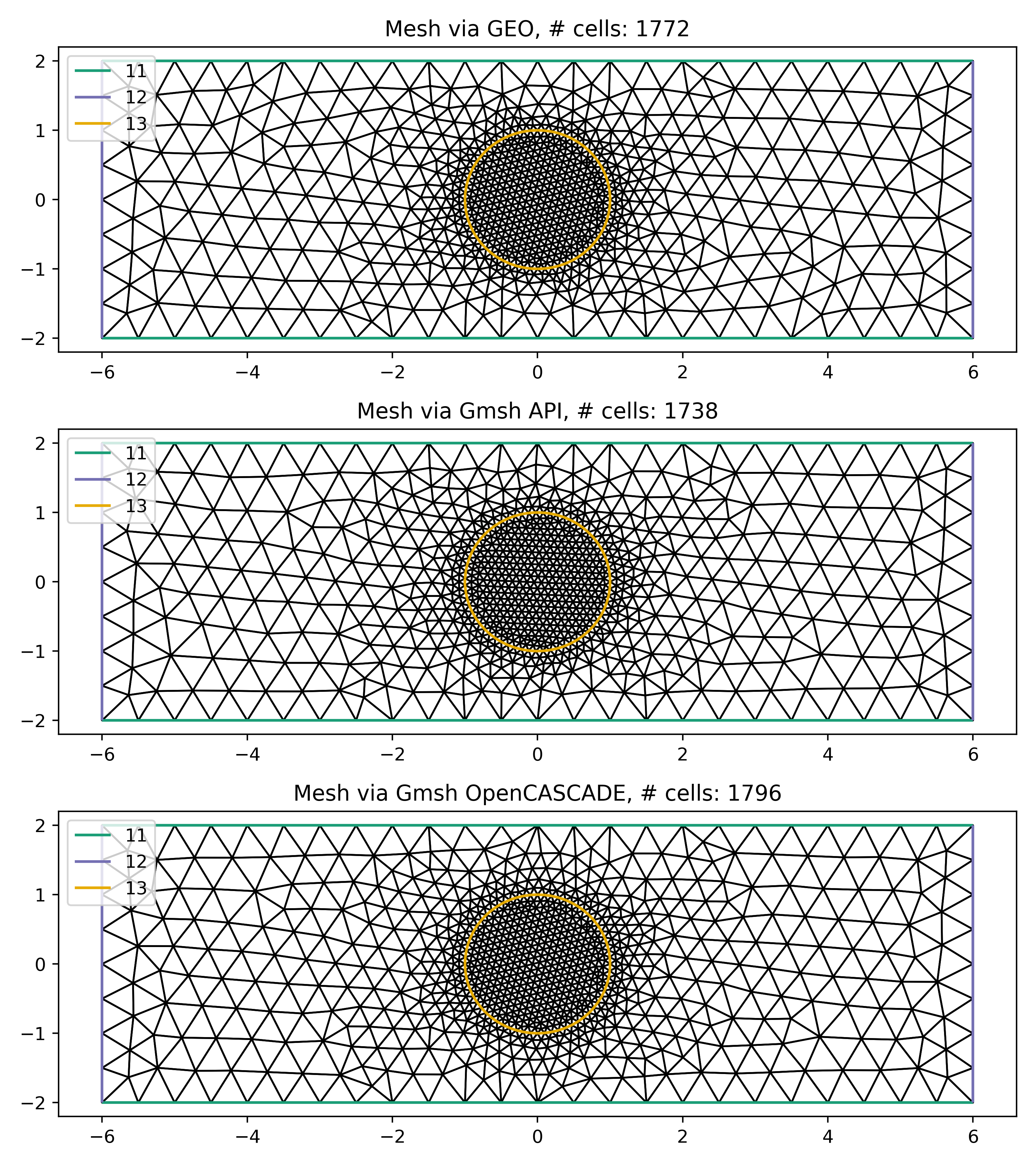
Compare Meshes
We can load and check the generated meshes in Firedrake.
meshes = [Mesh('gmsh_occ_demo.msh', name = "Gmsh API"),
          Mesh('gmsh_api_demo.msh', name = "Gmsh OpenCASCADE")]
fig, ax = plt.subplots(len(meshes), 1, figsize = (8, len(meshes)*3), tight_layout=True)
for m, ax in zip(meshes, ax):
   triplot(m, axes=ax)
   ax.set_title(f'Mesh via {m.name}, # cells: {m.num_cells()}')
   ax.legend(loc='upper left')

fig.savefig("gmsh_demo.png", dpi = 400)
Illustrate Features
To illustrate how to access all these features within Firedrake, we consider the following interface problem. Denoting by \(\Omega\) the filled rectangle and by \(D\) the disc, we seek a function \(u\in H^1_0(\Omega)\) such that
where \(\sigma = 1\) in \(\Omega \setminus D\) and \(\sigma = 2\) in \(D\). Since \(\sigma\) attains different values across \(\partial D\), we need to prescribe the behavior of \(u\) across this interface. This is implicitly done by imposing \(u\in H^1_0(\Omega)\): the function \(u\) must be continuous across \(\partial \Omega\). This allows us to employ Lagrangian finite elements to approximate \(u\). However, we also need to specify the the jump of \(\sigma \nabla u \cdot \vec{n}\) on \(\partial D\). This term arises naturally in the weak formulation of the problem under consideration. In this demo we simply set
The resulting weak formulation reads as follows:
The following Firedrake code shows how to solve this variational problem using linear Lagrangian finite elements.
# load the mesh generated with Gmsh
mesh = Mesh('gmsh_occ_demo.msh')

# define the space of linear Lagrangian finite elements
V = FunctionSpace(mesh, "CG", 1)

# define the trial function u and the test function v
u = TrialFunction(V)
v = TestFunction(V)

# define the bilinear form of the problem under consideration
# to specify the domain of integration, the surface tag is specified in brackets after dx
# in this example, 3 is the tag of the rectangle without the disc, and 4 is the disc tag
a = 2*dot(grad(v), grad(u))*dx(4) + dot(grad(v), grad(u))*dx(3) + v*u*dx

# define the linear form of the problem under consideration
# to specify the boundary of the boundary integral, the boundary tag is specified after dS
# note the use of dS due to 13 not being an external boundary
# Since the dS integral is an interior one, we must restrict the
# test function: since the space is continuous, we arbitrarily pick
# the '+' side.
L = Constant(5.) * v * dx + Constant(3.)*v('+')*dS(13)

# set homogeneous Dirichlet boundary conditions on the rectangle boundaries
# the tag  11 referes to the horizontal edges, the tag 12 refers to the vertical edges
DirBC = DirichletBC(V, 0, [11, 12])

# define u to contain the solution to the problem under consideration
u = Function(V)

# solve the variational problem
solve(a == L, u, bcs=DirBC, solver_parameters={'ksp_type': 'cg'})
A python script version of this demo can be found here.