
Warning
You are reading a version of the website built against the unstable main branch. This content is liable to change without notice and may be inappropriate for your use case.
You can find the documentation for the current stable release here.
Adaptive eigenvalue problem on an L-shaped domain
This demo computes the lowest eigenvalue of the Dirichlet Laplacian on an L-shaped domain to within a guaranteed error tolerance using adaptive mesh refinement. The error estimate in the eigenvalue is based on solving the problem with two complementary discretisations: a conforming method naturally yields an upper bound, while the Crouzeix-Raviart non-conforming method yields a lower bound after postprocessing proposed by Carstensen & Gedicke. The demo also demonstrates that adaptive mesh refinement is strictly more efficient than uniform refinement, due to the singularity of the eigenfunction at the re-entrant corner.
The demo was contributed by Patrick Farrell.
We consider the Dirichlet eigenvalue problem for the Poisson equation on an L-shaped domain \(\Omega\):
We aim to compute the lowest eigenvalue. Since the domain has a re-entrant corner, the eigenfunction has a singularity. Thus, uniform mesh refinement leads to suboptimal convergence. We demonstrate an adaptive strategy driven by a residual-based a posteriori error estimator. To establish rigorous bounds on the true eigenvalue \(\lambda\), we use conforming elements (CG) for an upper bound [Bof10], and nonconforming elements (CR) with Carstensen-Gedicke postprocessing [CG14] for a guaranteed lower bound.
We start by importing the necessary libraries:
from firedrake import *
from netgen.occ import *
We then define the L-shaped domain using Netgen’s Open CASCADE technology (OCC) interface, and generate an initial mesh:
rect1 = WorkPlane(Axes((0,0,0), n=Z, h=X)).Rectangle(1,2).Face()
rect2 = WorkPlane(Axes((0,1,0), n=Z, h=X)).Rectangle(2,1).Face()
L = rect1 + rect2

geo = OCCGeometry(L, dim=2)
ngmesh = geo.GenerateMesh(maxh=0.5)
mesh = Mesh(ngmesh)
We create a function to solve the eigenvalue problem for both continuous (CG) and nonconforming Crouzeix-Raviart (CR) [CR73] elements. By the Rayleigh-Ritz principle [Bof10, GW12], the CG solution provides an upper bound \(\lambda_{\text{ub}}\). The CR solution gives a discrete eigenvalue \(\lambda_{\text{CR}}\), which can be postprocessed to yield a guaranteed lower bound:
where \(\kappa_{\text{CR}} \approx 0.1893\) is the constant established by Carstensen and Gedicke [CG14]. A general theory for deriving lower bounds for eigenvalues with nonconforming methods has been developed by Hu et al. [HHL14]. We will use the postprocessed lower bound to terminate the adaptive iteration, while for technical reasons we will plot the Galerkin gap \(\lambda_{\text{CG}} - \lambda_{\text{CR}}\) to demonstrate optimal convergence.
To efficiently compute the smallest eigenvalue, we configure SLEPc using a solver parameters dictionary. We specify a Krylov-Schur eigensolver (eps_type) and a shift-and-invert spectral transformation (st_type) with a target of zero (eps_target). We also flag the generalized eigenvalue problem as Hermitian (eps_gen_hermitian) and request the smallest real eigenvalue (eps_smallest_real).
def solve_eigenproblem(mesh):
    h_symbolic = CellDiameter(mesh)
    DG0 = FunctionSpace(mesh, "DG", 0)
    h_cell = Function(DG0).interpolate(h_symbolic)
    with h_cell.dat.vec_ro as hvec:
        h_max = hvec.max()[1]
    eigenfunction = None

    for space in ["CG", "CR"]:
        V = FunctionSpace(mesh, space, 1)

        u = TrialFunction(V)
        v = TestFunction(V)

        a = inner(grad(u), grad(v))*dx
        b = inner(u, v)*dx
        bc = DirichletBC(V, 0, "on_boundary")
        eigenproblem = LinearEigenproblem(a, b, bc)

        sp = {
              "eps_gen_hermitian": None,
              "eps_smallest_real": None,
              "eps_monitor_cancel": None,
              "eps_type": "krylovschur",
              "eps_target": 0,
              "st_type": "sinvert",
              }

        eigensolver = LinearEigensolver(eigenproblem, 1, solver_parameters=sp)
        eigensolver.solve()

        if space == "CR":
            lambda_CR = eigensolver.eigenvalue(0).real
            kappa_CR = 0.1893
            lambda_lb = lambda_CR / (1 + kappa_CR**2 * h_max**2 * lambda_CR)
        if space == "CG":
            lambda_ub = eigensolver.eigenvalue(0).real
            eigenfunction = eigensolver.eigenfunction(0)[0]

    eigenfunction.rename("Eigenfunction")
    return (lambda_lb, lambda_ub, lambda_CR, eigenfunction)
These bounds do not describe where the mesh should be refined so as to reduce the error. For this purpose we employ a standard residual-based a posteriori error estimator [DPR03, Lar00]. Note that this assumes there is a single eigenfunction associated with the lowest eigenvalue; if the eigenvalue were of higher multiplicity the estimator would need to consider the entire eigenspace [BG14].
def estimate_error(mesh, uh, lam):
    W = FunctionSpace(mesh, "DG", 0)
    eta_sq = Function(W)
    w = TestFunction(W)
    h = CellDiameter(mesh)
    n = FacetNormal(mesh)
    v = CellVolume(mesh)

    G = (
          inner(eta_sq / v, w)*dx
        - inner(h**2 * (lam*uh + div(grad(uh)))**2, w) * dx
        - inner(h('+')/2 * jump(grad(uh), n)**2, w('+')) * dS
        - inner(h('-')/2 * jump(grad(uh), n)**2, w('-')) * dS
        )

    sp = {"mat_type": "matfree", "ksp_type": "preonly", "pc_type": "jacobi"}
    solve(G == 0, eta_sq, solver_parameters=sp)
    eta = Function(W).interpolate(sqrt(eta_sq))

    with eta.dat.vec_ro as eta_:
        error_est = eta_.norm()
    return (eta, error_est)
We define a function to adapt the mesh by refining elements with large error indicators, using the maximum Dörfler-like marking strategy with \(\theta = 0.5\):
def adapt(mesh, eta):
    W = FunctionSpace(mesh, "DG", 0)
    markers = Function(W)

    with eta.dat.vec_ro as eta_:
        eta_max = eta_.max()[1]

    theta = 0.5
    should_refine = conditional(gt(eta, theta*eta_max), 1, 0)
    markers.interpolate(should_refine)

    return mesh.refine_marked_elements(markers)
Finally, we run the adaptive loop until the upper and lower bounds agree to within a tolerance.
max_iterations = 20
error_estimators = []
dofs = []
err = 1

for i in range(max_iterations):
    lam_lb, lam_ub, lam_CR, uh = solve_eigenproblem(mesh)
    err = lam_ub - lam_lb
    gap = lam_ub - lam_CR
    error_estimators.append(gap)
    dofs.append(uh.function_space().dim())
    print(f"Level {i}: Upper bound {lam_ub:.5f}, Lower bound {lam_lb:.5f}, Bound gap {err:.5e}, Galerkin gap {gap:.5e}")

    VTKFile(f"l_eigenfunction_{i}.pvd").write(uh)

    if err < 1e-2 or dofs[-1] > 1000000:
        break

    eta, _ = estimate_error(mesh, uh, lam_ub)
    mesh = adapt(mesh, eta)
To demonstrate that adaptivity is necessary to achieve the optimal convergence rate, we can run the same script with \(\theta = 0\), which forces uniform refinement (all cells are marked for refinement at every step). We make this optional by guarding it behind the Boolean run_uniform.
run_uniform = True

if run_uniform:
    mesh_uniform = Mesh(ngmesh)
    uniform_error_estimators = []
    uniform_dofs = []

    def adapt_uniform(mesh, eta):
        markers = Function(FunctionSpace(mesh, "DG", 0)).assign(1.0)
        return mesh.refine_marked_elements(markers)

    for i in range(max_iterations):
        lam_lb, lam_ub, lam_CR, uh = solve_eigenproblem(mesh_uniform)
        err = lam_ub - lam_lb
        gap = lam_ub - lam_CR
        uniform_error_estimators.append(gap)
        uniform_dofs.append(uh.function_space().dim())
        if err < 5e-3 or uniform_dofs[-1] > 1000000:
            break
        eta, _ = estimate_error(mesh_uniform, uh, lam_ub)
        mesh_uniform = adapt_uniform(mesh_uniform, eta)
We can plot the convergence of the Galerkin gap \(\lambda_{\text{ub}} - \lambda_{\text{CR}}\) against the number of degrees of freedom. With adaptivity, we achieve the optimal \(O(N^{-1})\) convergence rate. For uniform refinement, the error is initially dominated by the smooth part of the solution (yielding a pre-asymptotic \(O(N^{-1})\) rate), but as the mesh is refined, the singularity inevitably dominates and limits the asymptotic convergence to the suboptimal rate of \(O(N^{-2/3})\).
try:
    import matplotlib.pyplot as plt
    import numpy as np

    plt.grid()
    plt.loglog(dofs, error_estimators, '-ok', label=r"Adaptive refinement ($\theta = 0.5$)")
    scaling = error_estimators[0] / dofs[0]**-1
    plt.loglog(dofs, np.array(dofs)**(-1.0) * scaling, '--', label="Optimal convergence $N^{-1}$")

    if run_uniform:
        plt.loglog(uniform_dofs, uniform_error_estimators, '-or', label=r"Uniform refinement ($\theta = 0$)")
        scaling_uniform = uniform_error_estimators[-1] / uniform_dofs[-1]**(-2.0/3.0)
        plt.loglog(uniform_dofs, np.array(uniform_dofs)**(-2.0/3.0) * scaling_uniform, ':r', label=r"Suboptimal convergence $N^{-2/3}$")
    plt.xlabel("Number of degrees of freedom $N$")
    plt.ylabel(r"Galerkin gap $\lambda_{\text{ub}} - \lambda_{\text{CR}}$")
    plt.legend()
    plt.savefig("adaptive_eigenvalue_convergence.png")
except ImportError:
    warning("Matplotlib not imported")
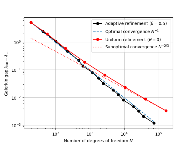
Convergence of the Galerkin gap \(\lambda_{\text{ub}} - \lambda_{\text{CR}}\). Note that the adaptive scheme achieves the optimal convergence rate of \(O(N^{-1})\), whereas uniform refinement is limited to the suboptimal rate of \(O(N^{-2/3})\).
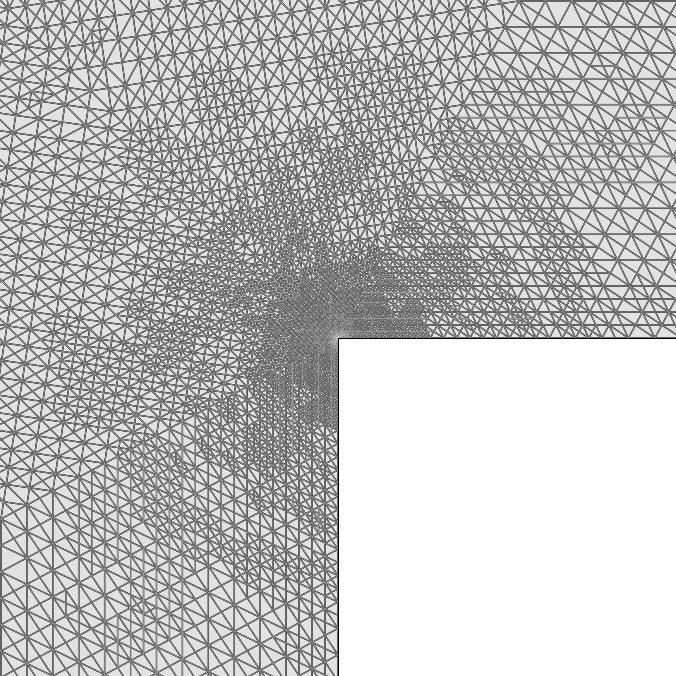
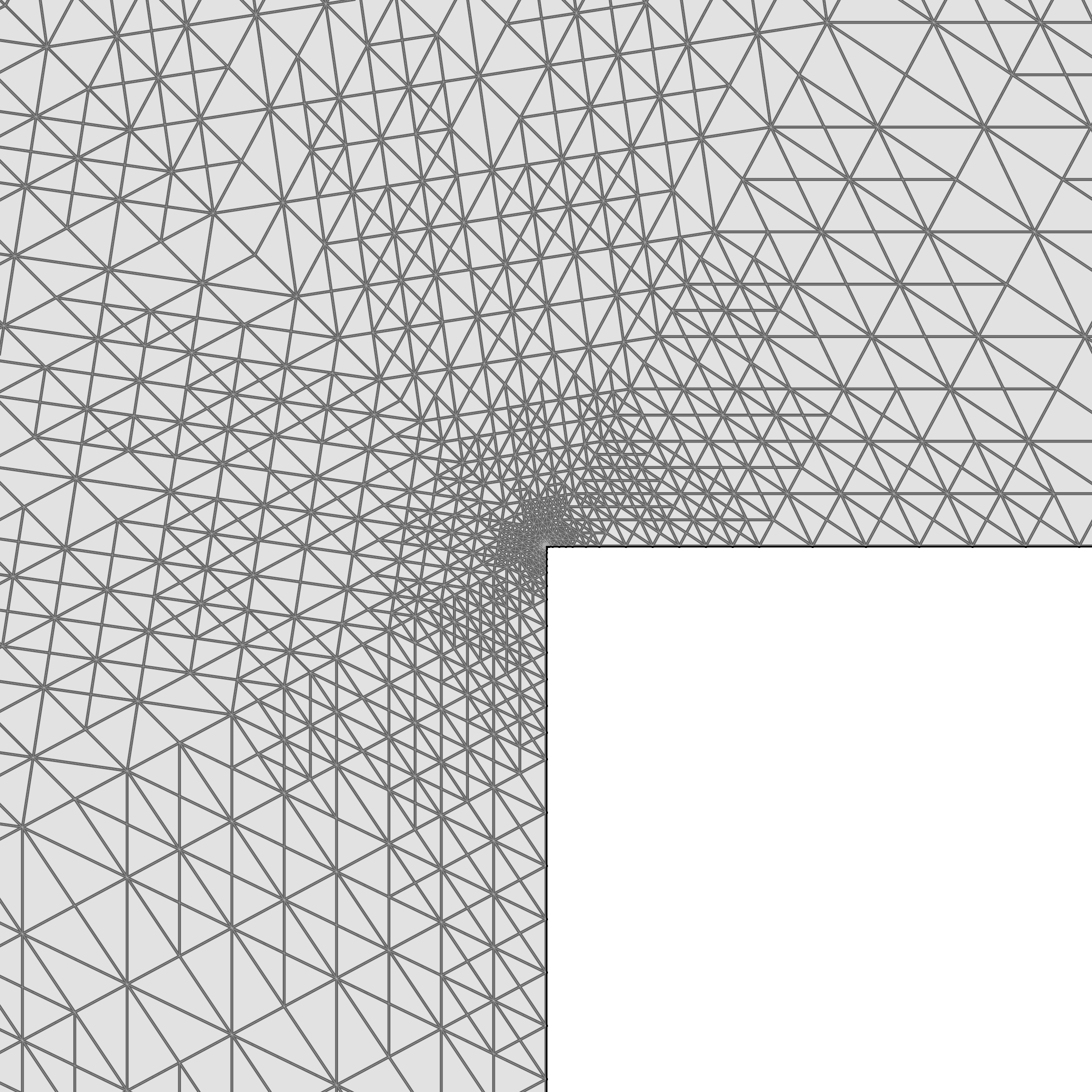
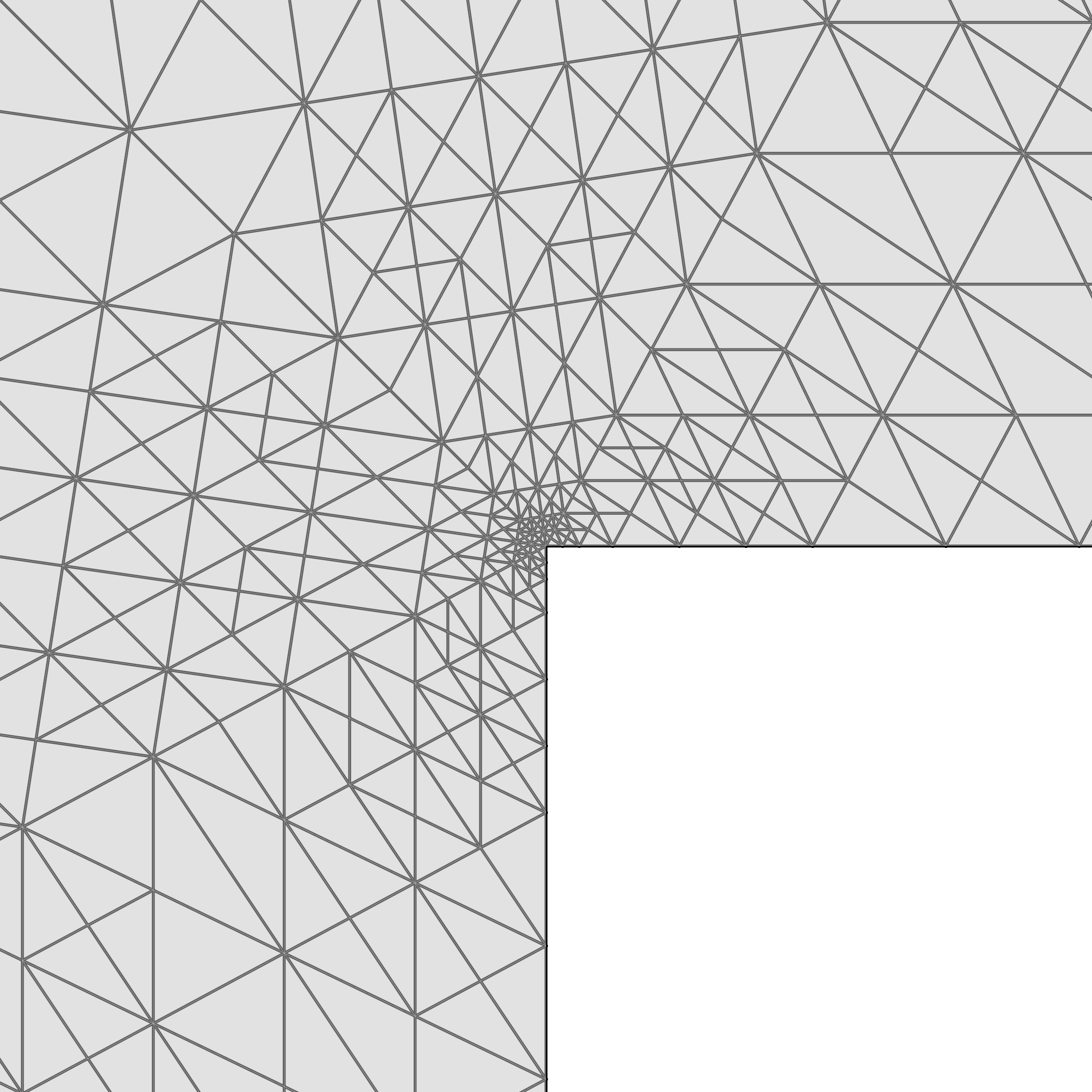
To visualize how the adaptive algorithm resolves the singularity, the sequence of images below shows the mesh (at refinement level 15), zooming into the re-entrant corner at 10x, 100x, and 1000x magnification.
References
Daniele Boffi. Finite element approximation of eigenvalue problems. Acta Numerica, 19:1–120, 2010. doi:10.1017/S0962492910000012.
Daniele Boffi and Lucia Gastaldi. Some remarks on finite element approximation of multiple eigenvalues. Applied Numerical Mathematics, 79:18–28, 2014. doi:10.1016/j.apnum.2012.08.006.
Carsten Carstensen and Joscha Gedicke. Guaranteed lower bounds for eigenvalues. Mathematics of Computation, 83(290):2605–2629, 2014. doi:10.1090/S0025-5718-2014-02833-0.
Michel Crouzeix and Pierre-Arnaud Raviart. Conforming and nonconforming finite element methods for solving the stationary Stokes equations I. Revue française d'automatique informatique recherche opérationnelle, 7(R3):33–75, 1973. doi:10.1051/m2an/197307r300331.
Ricardo G. Durán, Claudio Padra, and Rodolfo Rodríguez. A posteriori error estimates for the finite element approximation of eigenvalue problems. Mathematical Models and Methods in Applied Sciences, 13(8):1219–1229, 2003. doi:10.1142/S0218202503002878.
Martin J. Gander and Gerhard Wanner. From Euler, Ritz, and Galerkin to modern computing. SIAM Review, 54(4):627–666, 2012. doi:10.1137/100804036.
Jun Hu, Yunqing Huang, and Qun Lin. Lower bounds for eigenvalues of elliptic operators: by nonconforming finite element methods. Journal of Scientific Computing, 61(1):196–221, 2014. doi:10.1007/s10915-014-9821-5.
Mats G. Larson. A posteriori and a priori error analysis for finite element approximations of self-adjoint elliptic eigenvalue problems. SIAM Journal on Numerical Analysis, 38(2):608–625, 2000. doi:10.1137/S0036142997320164.