Visualising the results of simulations ¶

Having run a simulation, it is likely that we will want to look at the results. To do this, Firedrake supports saving data in VTK format, suitable for visualisation in Paraview (amongst others).

In addition, 1D and 2D function could be plotted and displayed using the python library of matplotlib (an optional dependency of firedrake)

Creating output files ¶

Output for visualisation purposes is managed with a VTKFile object. To create one, first import the class from firedrake.output, then we just need to pass the name of the output file on disk. The file Firedrake creates is in PVD_ and therefore the requested file name must end in `.pvd``.

outfile = VTKFile("output.pvd")
# The following raises an error
badfile = VTKFile("output.vtu")

To save functions to the VTKFile we use the write() method.

mesh = UnitSquareMesh(1, 1)
V = FunctionSpace(mesh, "DG", 0)
f = Function(V)
f.interpolate(sin(SpatialCoordinate(mesh)[0]))

outfile = VTKFile("output.pvd")
outfile.write(f)

Note

Output created for visualisation purposes is not intended for purposes other than visualisation. If you need to save data for checkpointing purposes, you should instead use Firedrake’s checkingpointing capabilities.

Saving time-dependent data ¶

Often, we have a time-dependent simulation and would like to save the same function at multiple timesteps. This is straightforward, we must create the output VTKFile outside the time loop and call write() inside.

...
outfile = VTKFile("timesteps.pvd")

while t < T:
    ...
    outfile.write(f)
    t += dt

The PVD data format supports specifying the timestep value for time-dependent data. We do not have to provide it to write(), by default an integer counter is used that is incremented by 1 each time write() is called. It is possible to override this by passing the keyword argument time.

...
outfile = VTKFile("timesteps.pvd")

while t < T:
    ...
    outfile.write(f, time=t)
    t += dt

Visualising high-order data ¶

The file format Firedrake outputs to currently supports the visualisation of scalar-, vector-, or tensor-valued fields represented with an arbitrary order (possibly discontinuous) Lagrange basis. Furthermore, the fields must be in an isoparametric function space, meaning the mesh coordinates associated to a field must be represented with the same basis as the field. To visualise fields in anything other than these spaces we must transform the data to this format first. One option is to do so by hand before outputting. Either by interpolating or else projecting the mesh coordinates and then the field. Since this is such a common operation, the VTKFile object is set up to manage these operations automatically, we just need to choose whether we want data to be interpolated or projected. The default is to use interpolation. For example, assume we wish to output a vector-valued function that lives in an \(H(\operatorname{div})\) space. If we want it to be interpolated in the output file we can use

V = FunctionSpace(mesh, "RT", 2)
f = Function(V)
...
outfile = VTKFile("output.pvd")
outfile.write(f)

If instead we want projection, we use

projected = VTKFile("proj_output.pvd", project_output=True)
projected.write(f)

Note

This feature requires Paraview version 5.5.0 or better. If you must use an older version of Paraview, you must manually interpolate mesh coordinates and field coordinates to a piecewise linear function space, represented with either a Lagrange (H1) or discontinuous Lagrange (L2) basis. The VTKFile is also setup to manage this issue. For instance, we can force the output to be discontinuous piecewise linears via

projected = VTKFile("proj_output.pvd", target_degree=1, target_continuity=H1)
projected.write(f)

Using Paraview on higher order data ¶

Paraview’s visualisation algorithims are typically exact on piecewise linear data, but if you write higher order data, Paraview will produce an approximate visualisation. This approximation can be controlled in at least two ways:

Under the display properties of an unstructured grid, the Nonlinear Subdivision Level can be increased; this option controls the display of unstructured grid data and can be used to present a plausible curved geometry. Further, the Nonlinear Subdivision Level can also be changed after applying filters such as Extract Surface.
The Tessellate filter can be applied to unstructured grid data and has three parameters: Chord Error, Maximum Number of Subdivisions, and Field Error. Tessellation is the process of approximating a higher order geometry via subdividing cells into smaller linear cells. Chord Error is a tessellation error metric, the distance between the midpoint of any edge on the tessellated geometry and a corresponding point in the original geometry. Field Error is analogous to Chord Error: the error of the field on the tessellated data is compared pointwise to the original data at the midpoints of the edges of the tessellated geometry and the corresponding points on the original geometry. The Maximum Number of Subdivisions is the maximum number of times an edge in the original geometry can be subdivided.

Besides the two tools listed above, Paraview provides many other tools (filters) that might be applied to the original data or composed with the tools listed above. Documentation on these interactions is sparse, but tessellation can be used to understand this issue: the Tessellate filter produces another unstructured grid from its inputs so algorithms can be applied to both the tessellated and input unstructured grid. The tessellated data can also be saved for future reference.

Note

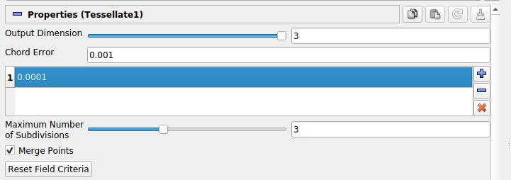
Field Error is hidden in the current Paraview UI (5.7) so we include a visual guide wherein the field error is set via the highlighted field directly below Chord Error:

We also note that the Tessellate filter (and other filters) can be more clearly controlled via the Paraview Python shell (under the View menu). For instance, Field Error can be more clearly specified via an argument to the Tessellate filter constructor.

from paraview.simple import *
pvd = PVDReader(FileName="Example.pvd")
tes = Tessellate(pvd, FieldError=0.001)

Saving multiple functions ¶

Often we will want to save, and subsequently visualise, multiple different fields from a simulation. For example the velocity and pressure in a fluids models. This is possible either by having a separate output file for each field, or by saving multiple fields to the same output file. The latter may be more convenient for subsequent analysis. To do this, we just need to pass multiple Functions to write().

u = Function(V, name="Velocity")
p = Function(P, name="Pressure")

outfile = VTKFile("output.pvd")

outfile.write(u, p, time=0)

# We can happily do this in a timeloop as well.
while t < t:
    ...
    outfile.write(u, p, time=t)

Note

Subsequent writes to the same file must use the same number of functions, and the functions must have the same names. The following example results in an error.

u = Function(V, name="Velocity")
p = Function(P, name="Pressure")

outfile = VTKFile("output.pvd")

outfile.write(u, p, time=0)
...
# This raises an error
outfile.write(u, time=1)
# as does this
outfile.write(p, u, time=1)

Selecting the output space when outputting multiple functions ¶

All functions, including the mesh coordinates, that are output to the same file must be represented in the same space, the rules for selecting the output space are as follows. First, all functions must be defined via the same cell type otherwise an exception will be thrown. Second, if all functions are continuous (i.e. they live in \(H^1\)), then the output space will be a piecewise continuous space. If any of the functions are at least partially discontinuous, again including the coordinate field (this occurs when using periodic meshes), then the output will use a piecewise discontinuous space. Third, the degree of the basis will be the maximum degree used over the spaces of all input functions. For elements where the degree is a tuple (this occurs when using tensor product elements), the the maximum will be over the elements of the tuple too, meaning a tensor product of elements of degree 4 and 2 will be turned into a tensor product of elements of degree 4 and 4.

Plotting with matplotlib ¶

Firedrake includes support for plotting meshes and functions using matplotlib. The API for plotting mimics that of matplotlib as much as possible. For example the functions tripcolor, tricontour, and so forth, all behave more or less like their counterparts in matplotlib, and actually call them under the hood. The only difference is that the Firedrake functions include an extra optional argument axes to specify the matplotlib Axes object to draw on. When using matplotlib by itself these methods are methods of the Axes object. Otherwise the usage is identical. For example, the following code would make a filled contour plot of the function u using the inferno colormap, with contours drawn at 0.0, 0.02, …, 1.0, and add a colorbar to the figure.

import matplotlib.pyplot as plt
import numpy as np
from firedrake import *
from firedrake.pyplot import tricontourf

mesh = UnitSquareMesh(10, 10)
V = FunctionSpace(mesh, "CG", 1)
u = Function(V)
x = SpatialCoordinate(mesh)
u.interpolate(x[0] + x[1])
fig, axes = plt.subplots()
levels = np.linspace(0, 1, 51)
contours = tricontourf(u, levels=levels, axes=axes, cmap="inferno")
axes.set_aspect("equal")
fig.colorbar(contours)
fig.show()

For vector fields, triplot and tricontour will show the magnitude of function. To see the direction as well, you can instead call the quiver function, which again works the same as its counterpart in matplotlib.

The function triplot has one major departure from matplotlib to make finite element analysis easier. The different segments of the boundary are shown with different colors in order to make it easy to determine the numeric ID of each boundary segment. Mistaking which segments of the boundary should have Dirichlet or Neumann boundary conditions is a common source of errors in applications. To see a legend explaining the colors, you can add a legend like so:

import matplotlib.pyplot as plt
from firedrake import *
from firedrake.pyplot import triplot

mesh = Mesh(mesh_filename)
fig, axes = plt.subplots()
triplot(mesh, axes=axes)
axes.legend()
fig.show()

The numeric IDs shown in the legend are the same as those stored internally in the mesh, so for example if you added physical lines using gmsh the numbering is the same.

For 1D functions with degree less than 4, the plot of the function would be exact using Bezier curves. For higher order 1D functions, the plot would be the linear approximation by sampling points of the function. The number of sample points per element could be specfied to when calling plot.

To install matplotlib, please look at the installation instructions of matplotlib.