
Adaptive eigenvalue problem on an L-shaped domain
This demo computes the lowest eigenvalue of the Dirichlet Laplacian on an L-shaped domain to within a guaranteed error tolerance using adaptive mesh refinement. The error estimate in the eigenvalue is based on solving the problem with two complementary discretisations: a conforming method naturally yields an upper bound, while the Crouzeix-Raviart non-conforming method yields a lower bound after postprocessing proposed by Carstensen & Gedicke. The demo also demonstrates that adaptive mesh refinement is strictly more efficient than uniform refinement, due to the singularity of the eigenfunction at the re-entrant corner.
The demo was contributed by Patrick Farrell.
We consider the Dirichlet eigenvalue problem for the Poisson equation on an L-shaped domain \(\Omega\):
We aim to compute the lowest eigenvalue. Since the domain has a re-entrant corner, the eigenfunction has a singularity. Thus, uniform mesh refinement leads to suboptimal convergence. We demonstrate an adaptive strategy driven by a residual-based a posteriori error estimator. To establish rigorous bounds on the true eigenvalue \(\lambda\), we use conforming elements (CG) for an upper bound [Bof10], and nonconforming elements (CR) with Carstensen-Gedicke postprocessing [CG14] for a guaranteed lower bound.
We start by importing the necessary libraries:
from firedrake import *
from netgen.occ import *
We then define the L-shaped domain using Netgen’s Open CASCADE technology (OCC) interface, and generate an initial mesh:
rect1 = WorkPlane(Axes((0,0,0), n=Z, h=X)).Rectangle(1,2).Face()
rect2 = WorkPlane(Axes((0,1,0), n=Z, h=X)).Rectangle(2,1).Face()
L = rect1 + rect2

geo = OCCGeometry(L, dim=2)
ngmesh = geo.GenerateMesh(maxh=0.5)
mesh = Mesh(ngmesh)
We create a function to solve the eigenvalue problem for both continuous (CG) and nonconforming Crouzeix-Raviart (CR) [CR73] elements. By the Rayleigh-Ritz principle [Bof10, GW12], the CG solution provides an upper bound \(\lambda_{\text{ub}}\). The CR solution gives a discrete eigenvalue \(\lambda_{\text{CR}}\), which can be postprocessed to yield a guaranteed lower bound:
where \(\kappa_{\text{CR}} \approx 0.1893\) is the constant established by Carstensen and Gedicke [CG14]. A general theory for deriving lower bounds for eigenvalues with nonconforming methods has been developed by Hu et al. [HHL14]. We will use the postprocessed lower bound to terminate the adaptive iteration, while for technical reasons we will plot the Galerkin gap \(\lambda_{\text{CG}} - \lambda_{\text{CR}}\) to demonstrate optimal convergence.
To efficiently compute the smallest eigenvalue, we configure SLEPc using a solver parameters dictionary. We specify a Krylov-Schur eigensolver (eps_type) and a shift-and-invert spectral transformation (st_type) with a target of zero (eps_target). We also flag the generalized eigenvalue problem as Hermitian (eps_gen_hermitian) and request the smallest real eigenvalue (eps_smallest_real).
def solve_eigenproblem(mesh):
    h_symbolic = CellDiameter(mesh)
    DG0 = FunctionSpace(mesh, "DG", 0)
    h_cell = Function(DG0).interpolate(h_symbolic)
    with h_cell.dat.vec_ro as hvec:
        h_max = hvec.max()[1]
    eigenfunction = None

    for space in ["CG", "CR"]:
        V = FunctionSpace(mesh, space, 1)

        u = TrialFunction(V)
        v = TestFunction(V)

        a = inner(grad(u), grad(v))*dx
        b = inner(u, v)*dx
        bc = DirichletBC(V, 0, "on_boundary")
        eigenproblem = LinearEigenproblem(a, b, bc)

        sp = {
              "eps_gen_hermitian": None,
              "eps_smallest_real": None,
              "eps_monitor_cancel": None,
              "eps_type": "krylovschur",
              "eps_target": 0,
              "st_type": "sinvert",
              }

        eigensolver = LinearEigensolver(eigenproblem, 1, solver_parameters=sp)
        eigensolver.solve()

        if space == "CR":
            lambda_CR = eigensolver.eigenvalue(0).real
            kappa_CR = 0.1893
            lambda_lb = lambda_CR / (1 + kappa_CR**2 * h_max**2 * lambda_CR)
        if space == "CG":
            lambda_ub = eigensolver.eigenvalue(0).real
            eigenfunction = eigensolver.eigenfunction(0)[0]

    eigenfunction.rename("Eigenfunction")
    return (lambda_lb, lambda_ub, lambda_CR, eigenfunction)
These bounds do not describe where the mesh should be refined so as to reduce the error. For this purpose we employ a standard residual-based a posteriori error estimator [DPR03, Lar00]. Note that this assumes there is a single eigenfunction associated with the lowest eigenvalue; if the eigenvalue were of higher multiplicity the estimator would need to consider the entire eigenspace [BG14].
def estimate_error(mesh, uh, lam):
    W = FunctionSpace(mesh, "DG", 0)
    eta_sq = Function(W)
    w = TestFunction(W)
    h = CellDiameter(mesh)
    n = FacetNormal(mesh)
    v = CellVolume(mesh)

    G = (
          inner(eta_sq / v, w)*dx
        - inner(h**2 * (lam*uh + div(grad(uh)))**2, w) * dx
        - inner(h('+')/2 * jump(grad(uh), n)**2, w('+')) * dS
        - inner(h('-')/2 * jump(grad(uh), n)**2, w('-')) * dS
        )

    sp = {"mat_type": "matfree", "ksp_type": "preonly", "pc_type": "jacobi"}
    solve(G == 0, eta_sq, solver_parameters=sp)
    eta = Function(W).interpolate(sqrt(eta_sq))

    with eta.dat.vec_ro as eta_:
        error_est = eta_.norm()
    return (eta, error_est)
We define a function to adapt the mesh by refining elements with large error indicators, using the maximum Dörfler-like marking strategy with \(\theta = 0.5\):
def adapt(mesh, eta):
    W = FunctionSpace(mesh, "DG", 0)
    markers = Function(W)

    with eta.dat.vec_ro as eta_:
        eta_max = eta_.max()[1]

    theta = 0.5
    should_refine = conditional(gt(eta, theta*eta_max), 1, 0)
    markers.interpolate(should_refine)

    return mesh.refine_marked_elements(markers)
Finally, we run the adaptive loop until the upper and lower bounds agree to within a tolerance.
max_iterations = 20
error_estimators = []
dofs = []
err = 1

for i in range(max_iterations):
    lam_lb, lam_ub, lam_CR, uh = solve_eigenproblem(mesh)
    err = lam_ub - lam_lb
    gap = lam_ub - lam_CR
    error_estimators.append(gap)
    dofs.append(uh.function_space().dim())
    print(f"Level {i}: Upper bound {lam_ub:.5f}, Lower bound {lam_lb:.5f}, Bound gap {err:.5e}, Galerkin gap {gap:.5e}")

    VTKFile(f"l_eigenfunction_{i}.pvd").write(uh)

    if err < 1e-2 or dofs[-1] > 1000000:
        break

    eta, _ = estimate_error(mesh, uh, lam_ub)
    mesh = adapt(mesh, eta)
To demonstrate that adaptivity is necessary to achieve the optimal convergence rate, we can run the same script with \(\theta = 0\), which forces uniform refinement (all cells are marked for refinement at every step). We make this optional by guarding it behind the Boolean run_uniform.
run_uniform = True

if run_uniform:
    mesh_uniform = Mesh(ngmesh)
    uniform_error_estimators = []
    uniform_dofs = []

    def adapt_uniform(mesh, eta):
        markers = Function(FunctionSpace(mesh, "DG", 0)).assign(1.0)
        return mesh.refine_marked_elements(markers)

    for i in range(max_iterations):
        lam_lb, lam_ub, lam_CR, uh = solve_eigenproblem(mesh_uniform)
        err = lam_ub - lam_lb
        gap = lam_ub - lam_CR
        uniform_error_estimators.append(gap)
        uniform_dofs.append(uh.function_space().dim())
        if err < 5e-3 or uniform_dofs[-1] > 1000000:
            break
        eta, _ = estimate_error(mesh_uniform, uh, lam_ub)
        mesh_uniform = adapt_uniform(mesh_uniform, eta)
We can plot the convergence of the Galerkin gap \(\lambda_{\text{ub}} - \lambda_{\text{CR}}\) against the number of degrees of freedom. With adaptivity, we achieve the optimal \(O(N^{-1})\) convergence rate. For uniform refinement, the error is initially dominated by the smooth part of the solution (yielding a pre-asymptotic \(O(N^{-1})\) rate), but as the mesh is refined, the singularity inevitably dominates and limits the asymptotic convergence to the suboptimal rate of \(O(N^{-2/3})\).
try:
    import matplotlib.pyplot as plt
    import numpy as np

    plt.grid()
    plt.loglog(dofs, error_estimators, '-ok', label=r"Adaptive refinement ($\theta = 0.5$)")
    scaling = error_estimators[0] / dofs[0]**-1
    plt.loglog(dofs, np.array(dofs)**(-1.0) * scaling, '--', label="Optimal convergence $N^{-1}$")

    if run_uniform:
        plt.loglog(uniform_dofs, uniform_error_estimators, '-or', label=r"Uniform refinement ($\theta = 0$)")
        scaling_uniform = uniform_error_estimators[-1] / uniform_dofs[-1]**(-2.0/3.0)
        plt.loglog(uniform_dofs, np.array(uniform_dofs)**(-2.0/3.0) * scaling_uniform, ':r', label=r"Suboptimal convergence $N^{-2/3}$")
    plt.xlabel("Number of degrees of freedom $N$")
    plt.ylabel(r"Galerkin gap $\lambda_{\text{ub}} - \lambda_{\text{CR}}$")
    plt.legend()
    plt.savefig("adaptive_eigenvalue_convergence.png")
except ImportError:
    warning("Matplotlib not imported")
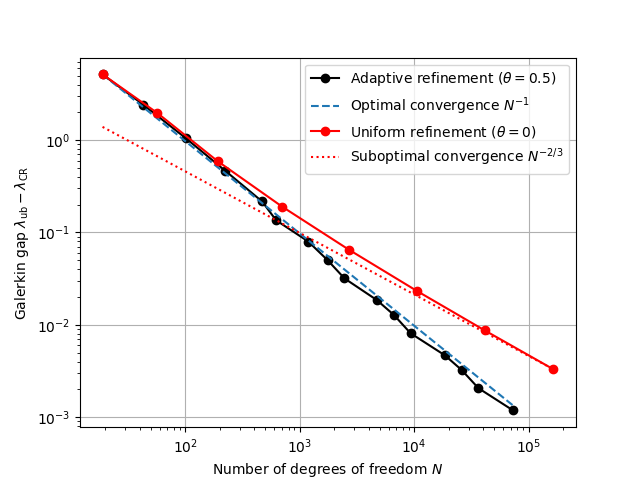
Convergence of the Galerkin gap \(\lambda_{\text{ub}} - \lambda_{\text{CR}}\). Note that the adaptive scheme achieves the optimal convergence rate of \(O(N^{-1})\), whereas uniform refinement is limited to the suboptimal rate of \(O(N^{-2/3})\).
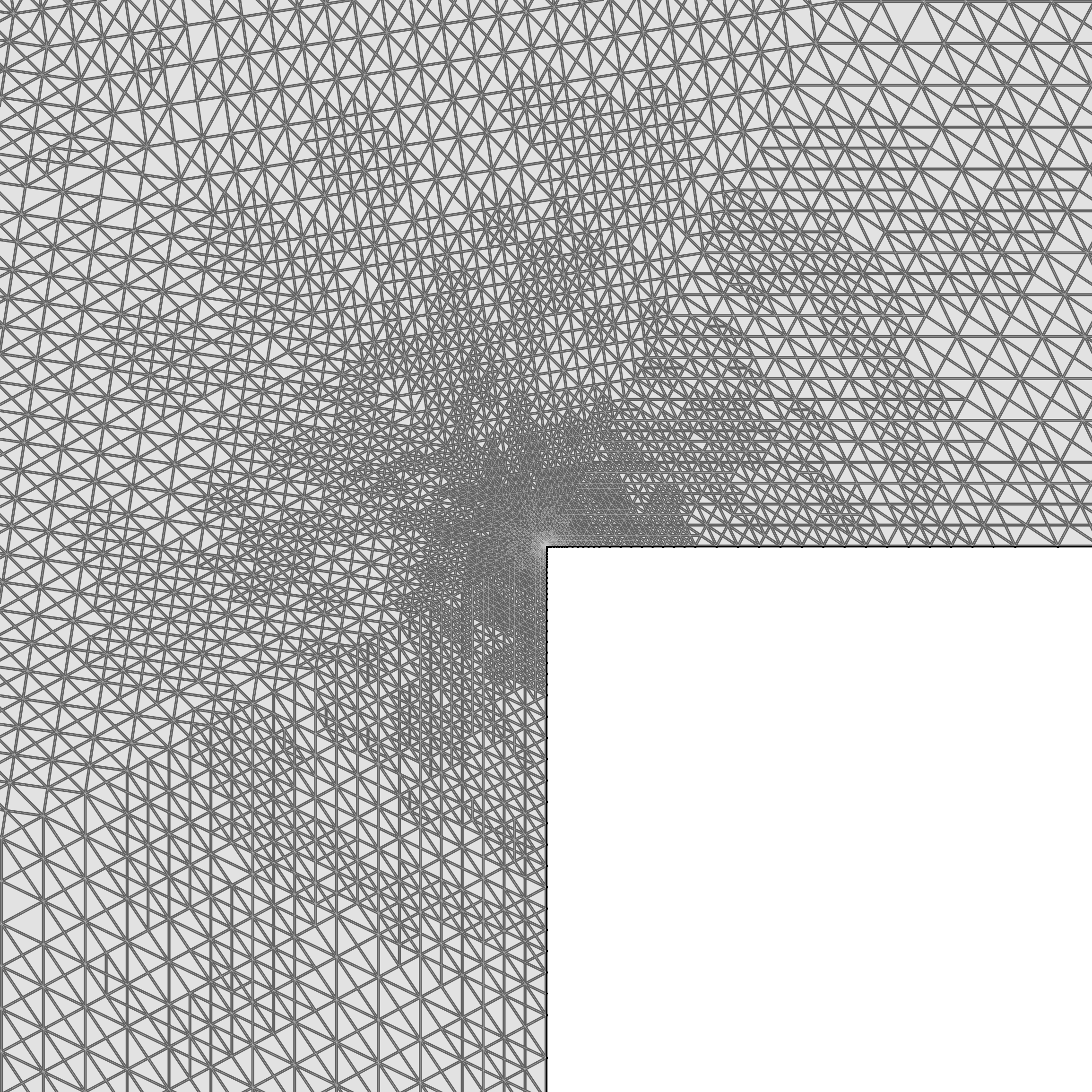
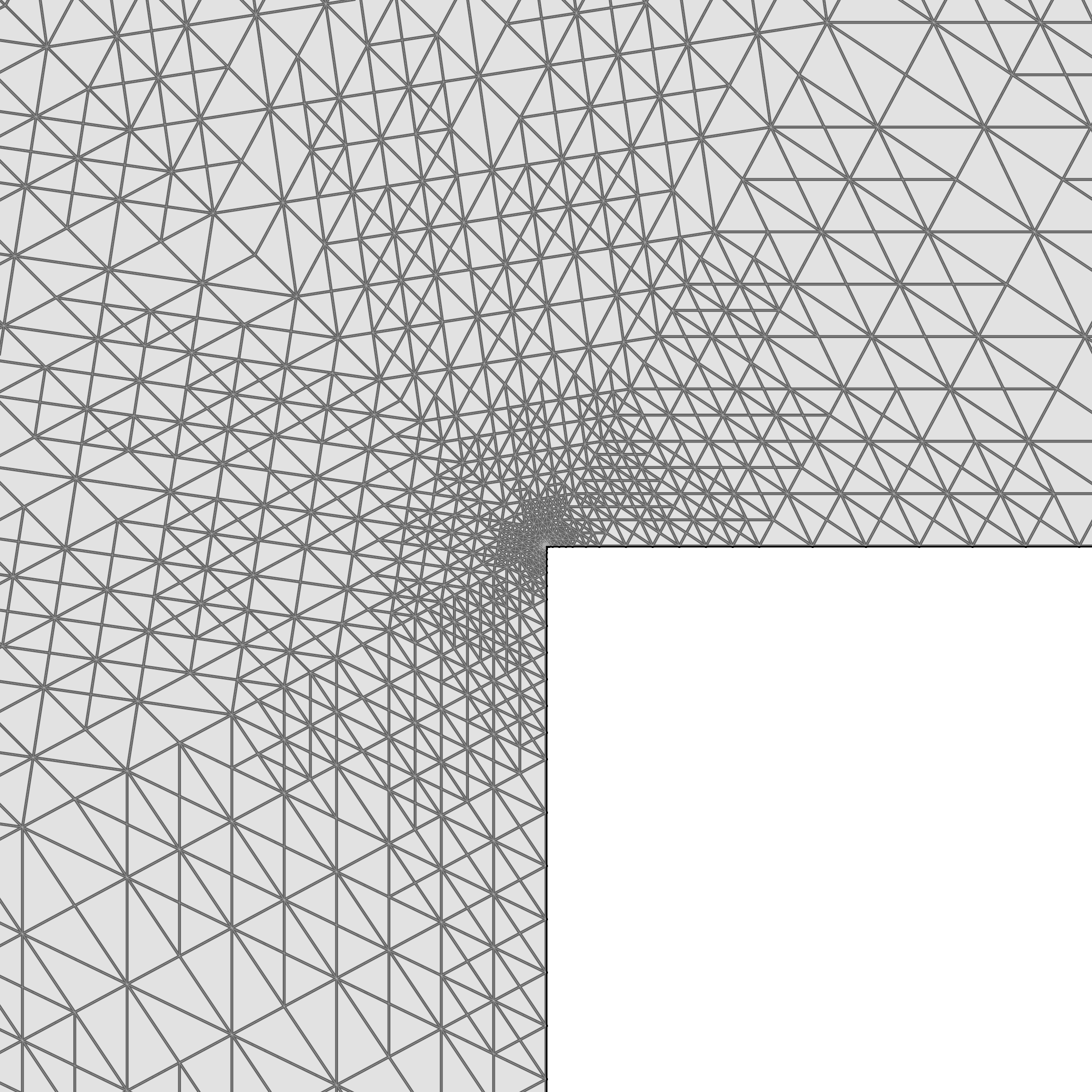
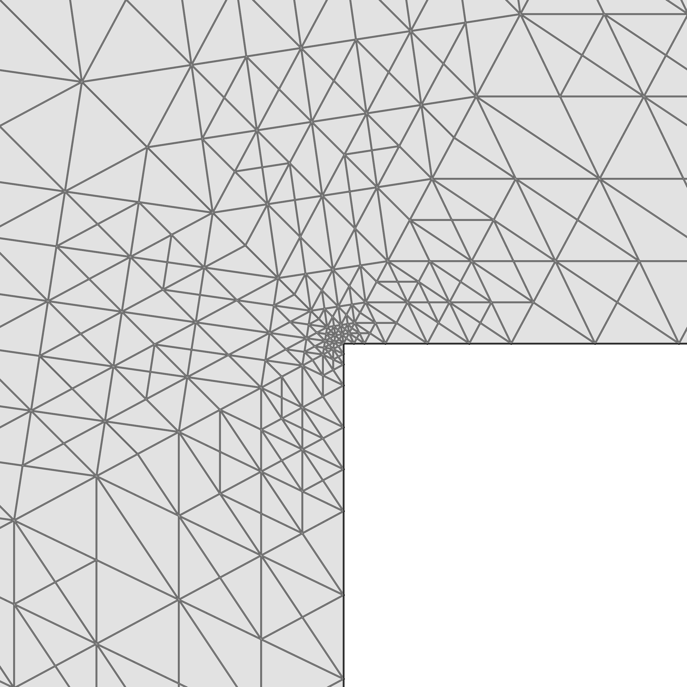
To visualize how the adaptive algorithm resolves the singularity, the sequence of images below shows the mesh (at refinement level 15), zooming into the re-entrant corner at 10x, 100x, and 1000x magnification.
References
Daniele Boffi. Finite element approximation of eigenvalue problems. Acta Numerica, 19:1–120, 2010. doi:10.1017/S0962492910000012.
Daniele Boffi and Lucia Gastaldi. Some remarks on finite element approximation of multiple eigenvalues. Applied Numerical Mathematics, 79:18–28, 2014. doi:10.1016/j.apnum.2012.08.006.
Carsten Carstensen and Joscha Gedicke. Guaranteed lower bounds for eigenvalues. Mathematics of Computation, 83(290):2605–2629, 2014. doi:10.1090/S0025-5718-2014-02833-0.
Michel Crouzeix and Pierre-Arnaud Raviart. Conforming and nonconforming finite element methods for solving the stationary Stokes equations I. Revue française d'automatique informatique recherche opérationnelle, 7(R3):33–75, 1973. doi:10.1051/m2an/197307r300331.
Ricardo G. Durán, Claudio Padra, and Rodolfo Rodríguez. A posteriori error estimates for the finite element approximation of eigenvalue problems. Mathematical Models and Methods in Applied Sciences, 13(8):1219–1229, 2003. doi:10.1142/S0218202503002878.
Martin J. Gander and Gerhard Wanner. From Euler, Ritz, and Galerkin to modern computing. SIAM Review, 54(4):627–666, 2012. doi:10.1137/100804036.
Jun Hu, Yunqing Huang, and Qun Lin. Lower bounds for eigenvalues of elliptic operators: by nonconforming finite element methods. Journal of Scientific Computing, 61(1):196–221, 2014. doi:10.1007/s10915-014-9821-5.
Mats G. Larson. A posteriori and a priori error analysis for finite element approximations of self-adjoint elliptic eigenvalue problems. SIAM Journal on Numerical Analysis, 38(2):608–625, 2000. doi:10.1137/S0036142997320164.