
Note
You can run this notebook on Google Colab.
HPC Demonstration
In this notebook we build up a multigrid solver for an elliptic problem specifically designed for running Firedrake on a High Performance Computer (HPC). We will solve very large instances of the Poisson problem, demonstrating a range of different solver options and assessing their performance for a range of problem sizes. Additional supplimentary material is provided for running scripts on HPC.
Note: The code in this notebook is designed to be run on a large HPC facility, as a result some cells may take a long time to run in an interactive notebook. We suggest not re-running the notebook cells, but instead trying the exercises on a supercomputer.
We start as always by importing Firedrake. We also define parprint to perform parallel printing as in this demonstration. The Python time module is imported to benchmark the different solvers.
[1]:
from firedrake import *
from firedrake.petsc import PETSc
from time import time

parprint = PETSc.Sys.Print
How big?
The parameters Nx, Nref and degree defined below have been selected so that the simulation runs on a single core in a notebook. This is not the regime we want to think about in this tutorial, we want to think about very large problems. We will consider how each of these parameters affects the overall problem size.
[2]:
Nx = 8
Nref = 2
degree = 2
These three parameters determine the total number of degrees of freedom (DOFs) in our problem:
Nxdefines our coarse grid in the mesh hierarchy, it is used to construct a coarse cube mesh.Nrefdetermines how many times the mesh is refined to create a mesh hierarchy.degree, which we denote \(k\), specifies the polynomial order of the basis functions used to approximate functions in our finite element space.
The total number of DOFs is given by:
where \(d=3\) is the dimension of the domain in which we solve the problem.
This small notebook example solves a problem with a large number of DOFs, but on HPC we want to solve problems orders of magnitude larger still, by the end of this notebook we will be considering problems larger than 30 000 000 DOFs.
When solving problems using Firedrake in parallel, it’s worth remembering that performance can be improved by adding more processes (MPI ranks) as long as the number of DOFs remains above 50 000 DOFs per core.
The equations
We will consider the Poisson equation in a 3D domain \(\Omega = [0, 1]^3\):
where \(f\) is given by:
We use this particular right hand side since it has corresponding analytic solution:
Having an analytic solution allows us to compute the error in our computed solution as \(e_h = \|u_h - u\|_{L^2}\). For this notebook we fix \(a=1\) and \(b=2\).
The Poisson equation has the weak form: Find \(u_h \in V\) such that
For the discrete function space \(V\) we initially consider piecewise quadratic Lagrange elements, that is
V = FunctionSpace(mesh, "CG", 2)
It is straightforward to solve the equation using Firedrake by expressing this weak form in UFL. The Python code below generates a problem object of the desired size, a function u_h to store the solution and the analytic solution truth so we can compute the \(L_2\) error norm, all of which we use throughout the rest of the notebook.
[3]:
# Create mesh and mesh hierarchy
mesh = UnitCubeMesh(Nx, Nx, Nx)
hierarchy = MeshHierarchy(mesh, Nref)
mesh = hierarchy[-1]

# Define the function space and print the DOFs
V = FunctionSpace(mesh, "Lagrange", degree)
dofs = V.dim()
parprint('DOFs', dofs)

u = TrialFunction(V)
v = TestFunction(V)

bcs = DirichletBC(V, zero(), ("on_boundary",))

# Define the RHS and analytic solution
x, y, z = SpatialCoordinate(mesh)

a = Constant(1)
b = Constant(2)
exact = sin(pi*x)*tan(pi*x/4)*sin(a*pi*y)*sin(b*pi*z)
truth = Function(V).interpolate(exact)
f = -pi**2 / 2
f *= 2*cos(pi*x) - cos(pi*x/2) - 2*(a**2 + b**2)*sin(pi*x)*tan(pi*x/4)
f *= sin(a*pi*y)*sin(b*pi*z)

# Define the problem using the bilinear form `a` and linear functional `L`
a = dot(grad(u), grad(v))*dx
L = f*v*dx
u_h = Function(V)
problem = LinearVariationalProblem(a, L, u_h, bcs=bcs)
DOFs 274625
Creating a problem instance we can see there are just short of 275000 DOFs in this noteook example.
The Solver
This table summarises the different solvers we will use:
Solver |
Abbreviation |
Cost |
Information |
|---|---|---|---|
LU |
LU |
O(n³)* |
Firedrake Default |
Conjugate Gradient + Algebraic Multigrid |
CG + AMG |
O(qn) |
Sensible choice of KSP + PC |
Conjugate Gradient + Geometric Multigrid V-cycle |
CG + GMG V-cycle |
O(qn) |
GMG in place of AMG |
Full Geometric Multigrid |
CG + Full GMG |
O(qn) |
|
Matrix free FMG with Telescoping |
Matfree CG + telescoped full GMG |
O(qn) |
Reduced memory and communication |
*See discussion at the end of the LU section
The n in the above table is the problem size (number of DOFs) and q is the number of iterations taken by an iterative method. In this notebook we use multigrid preconditioners to try and minimise the number of iterations, q.
We define a function to wrap the solve, so we can provide different solver options and to assess their performance, the run time is printed. This is a fairly crude way to profile our code, for a more in depth guide to profiling, take a look at the page on optimising Firedrake performance.
[4]:
def run_solve(problem, parameters):
    # Create a solver and time how long the solve takes
    t = time()
    solver = LinearVariationalSolver(problem, solver_parameters=parameters)
    solver.solve()
    parprint("Runtime :", time() - t)
LU
We can start by looking at the Firedrake’s default solver options. If you don’t specify any solver options a direct solver such as MUMPS will be used to perform an LU factorisation.
Here we explicitly list the PETSc solver options so it’s clear how the solver is set up. We also enable the snes_view so that PETSc prints the solver options it’s using at runtime.
Warning: This cell will take a long time (>2 minutes) to execute interactively!
[5]:
u_h.assign(0)
lu_mumps = {
    "snes_view": None,
    "ksp_type": "preonly",
    "pc_type": "lu",
    "pc_factor_mat_solver_type": "mumps"
}
run_solve(problem, lu_mumps)
parprint("Error   :", errornorm(truth, u_h))
SNES Object: (firedrake_0_) 1 MPI process
  type: ksponly
  maximum iterations=50, maximum function evaluations=10000
  tolerances: relative=1e-08, absolute=1e-50, solution=1e-08
  total number of linear solver iterations=1
  total number of function evaluations=1
  norm schedule ALWAYS
  KSP Object: (firedrake_0_) 1 MPI process
    type: preonly
    maximum iterations=10000, initial guess is zero
    tolerances: relative=1e-05, absolute=1e-50, divergence=10000.
    left preconditioning
    not checking for convergence
  PC Object: (firedrake_0_) 1 MPI process
    type: lu
      out-of-place factorization
      tolerance for zero pivot 2.22045e-14
      matrix ordering: external
      factor fill ratio given 0., needed 0.        Factored matrix:
          Mat Object: (firedrake_0_) 1 MPI process
            type: mumps
            rows=274625, cols=274625
            package used to perform factorization: mumps
            total: nonzeros=462157931, allocated nonzeros=462157931
              MUMPS run parameters:
                Use -firedrake_0_ksp_view ::ascii_info_detail to display information for all processes
                RINFOG(1) (global estimated flops for the elimination after analysis): 1.48637e+12
                RINFOG(2) (global estimated flops for the assembly after factorization): 1.03961e+09
                RINFOG(3) (global estimated flops for the elimination after factorization): 1.48637e+12
                (RINFOG(12) RINFOG(13))*2^INFOG(34) (determinant): (0.,0.)*(2^0)                INFOG(3) (estimated real workspace for factors on all processors after analysis): 462157931
                INFOG(4) (estimated integer workspace for factors on all processors after analysis): 3296826
                INFOG(5) (estimated maximum front size in the complete tree): 8513
                INFOG(6) (number of nodes in the complete tree): 9587
                INFOG(7) (ordering option effectively used after analysis): 4
                INFOG(8) (structural symmetry in percent of the permuted matrix after analysis): 100
                INFOG(9) (total real/complex workspace to store the matrix factors after factorization): 462157931
                INFOG(10) (total integer space store the matrix factors after factorization): 3296826
                INFOG(11) (order of largest frontal matrix after factorization): 8513
                INFOG(12) (number of off-diagonal pivots): 0
                INFOG(13) (number of delayed pivots after factorization): 0
                INFOG(14) (number of memory compress after factorization): 0
                INFOG(15) (number of steps of iterative refinement after solution): 0
                INFOG(16) (estimated size (in MB) of all MUMPS internal data for factorization after analysis: value on the most memory consuming processor): 4746
                INFOG(17) (estimated size of all MUMPS internal data for factorization after analysis: sum over all processors): 4746
                INFOG(18) (size of all MUMPS internal data allocated during factorization: value on the most memory consuming processor): 4746
                INFOG(19) (size of all MUMPS internal data allocated during factorization: sum over all processors): 4746
                INFOG(20) (estimated number of entries in the factors): 462157931
                INFOG(21) (size in MB of memory effectively used during factorization - value on the most memory consuming processor): 3975
                INFOG(22) (size in MB of memory effectively used during factorization - sum over all processors): 3975
                INFOG(23) (after analysis: value of ICNTL(6) effectively used): 0
                INFOG(24) (after analysis: value of ICNTL(12) effectively used): 1
                INFOG(25) (after factorization: number of pivots modified by static pivoting): 0
                INFOG(28) (after factorization: number of null pivots encountered): 0
                INFOG(29) (after factorization: effective number of entries in the factors (sum over all processors)): 462157931
                INFOG(30, 31) (after solution: size in Mbytes of memory used during solution phase): 4667, 4667
                INFOG(32) (after analysis: type of analysis done): 1
                INFOG(33) (value used for ICNTL(8)): 7
                INFOG(34) (exponent of the determinant if determinant is requested): 0
                INFOG(35) (after factorization: number of entries taking into account BLR factor compression - sum over all processors): 462157931
                INFOG(36) (after analysis: estimated size of all MUMPS internal data for running BLR in-core - value on the most memory consuming processor): 0
                INFOG(37) (after analysis: estimated size of all MUMPS internal data for running BLR in-core - sum over all processors): 0
                INFOG(38) (after analysis: estimated size of all MUMPS internal data for running BLR out-of-core - value on the most memory consuming processor): 0
                INFOG(39) (after analysis: estimated size of all MUMPS internal data for running BLR out-of-core - sum over all processors): 0
    linear system matrix, which is also used to construct the preconditioner:
    Mat Object: (firedrake_0_) 1 MPI process
      type: seqaij
      rows=274625, cols=274625
      total: nonzeros=7678721, allocated nonzeros=7678721
      total number of mallocs used during MatSetValues calls=0
        not using I-node routines
Runtime : 48.440492391586304
Error   : 1.7378060441770724e-05
The above solve takes under a minute on a single Zen2 core of ARCHER2.
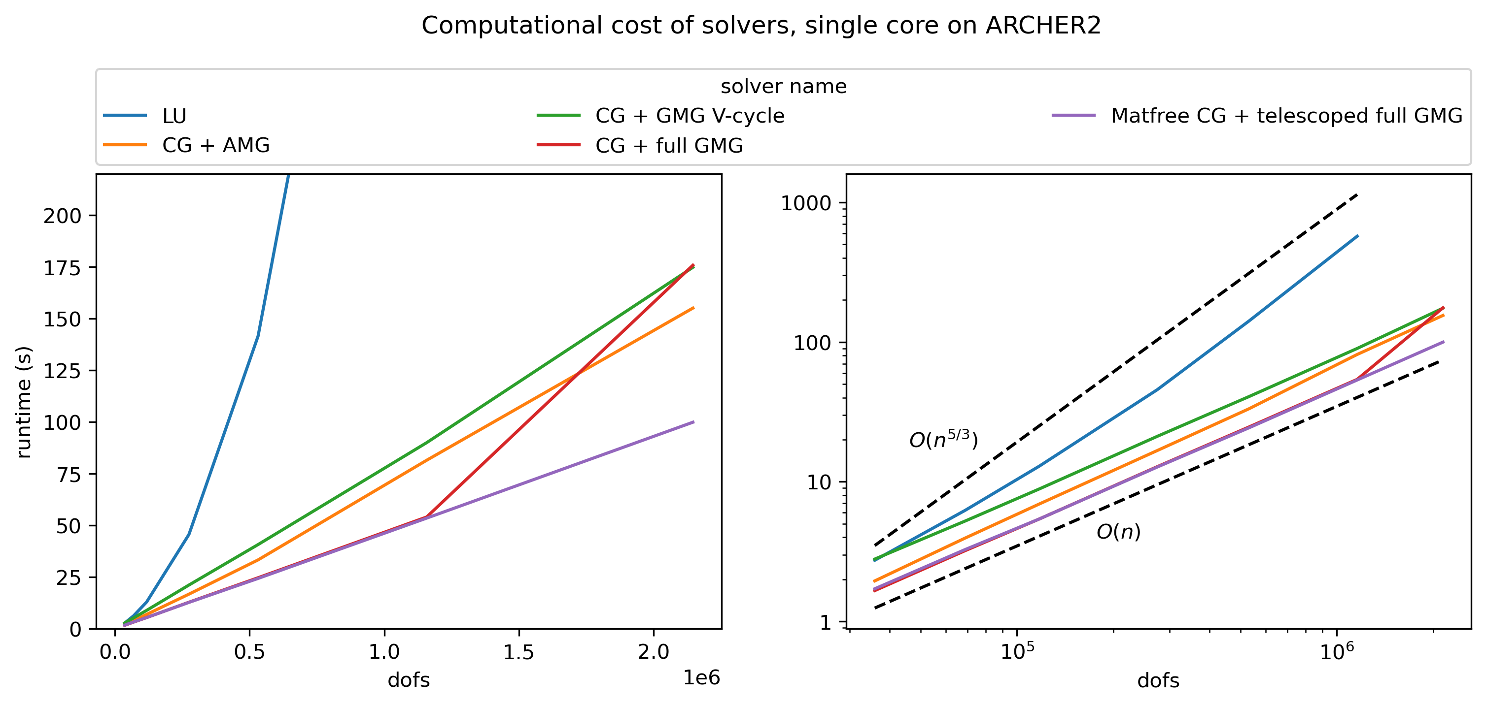
Dense LU factorisations are very expensive, typically \(O(n^3)\). Sparse LU with a state of the art solver like MUMPS or SuperLU_dist can do better, typically in \(O(n^2)\) for a 3D finite element matrix or \(O(n^{3/2})\) in 2D. For specific problems it may be possible to reduce that complexity even further.
We can measure the computational cost of our solvers by increasing the problem size (the number of DOFs) and observing how this changes the solver run time. In the computational cost plots below you can see that the cost of LU factorisation is approximately \(O(n^{5/3})\), but this cost grows far faster than the other solver methods.
Direct solvers are very fast for small problems, which is why LU is the default solver in Firedrake. However, when \(n\) gets large, direct solvers are no longer viable and should be avoided where possible.
Iterative solvers
An alternative to a direct solver is an iterative solver and PETSc gives us access to a large number of Krylov Subspace solvers (KSP). Since we have a symmetric problem, we can use the Conjugate Gradient (CG) method, which has computational cost \(O(qn)\), where \(q\) is the number of iterations for the method to converge.
To reduce \(q\) we can precondition the KSP, here we use PETSc’s gamg Algebraic Multigrid (AMG) as a preconditioner.
We assign 0 to the function u_h before we solve so that we aren’t using the solution from the LU solve above as our initial guess for the CG solver.
[6]:
u_h.assign(0)
cg_amg = {
    "snes_view": None,
    "ksp_type": "cg",
    "pc_type": "gamg",
    "pc_mg_log": None
}
run_solve(problem, cg_amg)
parprint("Error   :", errornorm(truth, u_h))
SNES Object: (firedrake_1_) 1 MPI process
  type: ksponly
  maximum iterations=50, maximum function evaluations=10000
  tolerances: relative=1e-08, absolute=1e-50, solution=1e-08
  total number of linear solver iterations=24
  total number of function evaluations=1
  norm schedule ALWAYS
  KSP Object: (firedrake_1_) 1 MPI process
    type: cg
    maximum iterations=10000, initial guess is zero
    tolerances: relative=1e-07, absolute=1e-50, divergence=10000.
    left preconditioning
    using PRECONDITIONED norm type for convergence test
  PC Object: (firedrake_1_) 1 MPI process
    type: gamg
      type is MULTIPLICATIVE, levels=4 cycles=v
        Cycles per PCApply=1
        Using externally compute Galerkin coarse grid matrices
        GAMG specific options
          Threshold for dropping small values in graph on each level =     -1.     -1.     -1.     -1.
          Threshold scaling factor for each level not specified = 1.
          AGG specific options
            Number of levels of aggressive coarsening 1
            Square graph aggressive coarsening
            MatCoarsen Object: (firedrake_1_) 1 MPI process
              type: misk
            Number smoothing steps to construct prolongation 1
          Complexity:    grid = 1.0133    operator = 1.02978
          Per-level complexity: op = operator, int = interpolation
              #equations  | #active PEs | avg nnz/row op | avg nnz/row int
                    8            1              8                0
                  167            1             73                6
                 3478            1             63                9
               274625            1             28                5
    Coarse grid solver -- level 0 -------------------------------
      KSP Object: (firedrake_1_mg_coarse_) 1 MPI process
        type: preonly
        maximum iterations=10000, initial guess is zero
        tolerances: relative=1e-05, absolute=1e-50, divergence=10000.
        left preconditioning
        not checking for convergence
      PC Object: (firedrake_1_mg_coarse_) 1 MPI process
        type: bjacobi
          number of blocks = 1
          Local solver information for first block is in the following KSP and PC objects on rank 0:
          Use -firedrake_1_mg_coarse_ksp_view ::ascii_info_detail to display information for all blocks
          KSP Object: (firedrake_1_mg_coarse_sub_) 1 MPI process
            type: preonly
            maximum iterations=1, initial guess is zero
            tolerances: relative=1e-05, absolute=1e-50, divergence=10000.
            left preconditioning
            not checking for convergence
          PC Object: (firedrake_1_mg_coarse_sub_) 1 MPI process
            type: lu
              out-of-place factorization
              tolerance for zero pivot 2.22045e-14
              using diagonal shift on blocks to prevent zero pivot [INBLOCKS]
              matrix ordering: nd
              factor fill ratio given 5., needed 1.
                Factored matrix:
                  Mat Object: (firedrake_1_mg_coarse_sub_) 1 MPI process
                    type: seqaij
                    rows=8, cols=8
                    package used to perform factorization: petsc
                    total: nonzeros=64, allocated nonzeros=64
                      using I-node routines: found 2 nodes, limit used is 5
            linear system matrix, which is also used to construct the preconditioner:
            Mat Object: (firedrake_1_mg_coarse_sub_) 1 MPI process
              type: seqaij
              rows=8, cols=8
              total: nonzeros=64, allocated nonzeros=64
              total number of mallocs used during MatSetValues calls=0
                using I-node routines: found 2 nodes, limit used is 5
        linear system matrix, which is also used to construct the preconditioner:
        Mat Object: (firedrake_1_mg_coarse_sub_) 1 MPI process
          type: seqaij
          rows=8, cols=8
          total: nonzeros=64, allocated nonzeros=64
          total number of mallocs used during MatSetValues calls=0
            using I-node routines: found 2 nodes, limit used is 5
    Down solver (pre-smoother) on level 1 -------------------------------
      KSP Object: (firedrake_1_mg_levels_1_) 1 MPI process
        type: chebyshev
          Chebyshev polynomial of first kind
          eigenvalue targets used: min 0.186657, max 2.05322
          eigenvalues provided (min 0.497524, max 1.86657) with transform: [0. 0.1; 0. 1.1]        maximum iterations=2, nonzero initial guess
        tolerances: relative=1e-05, absolute=1e-50, divergence=10000.
        left preconditioning
        not checking for convergence
      PC Object: (firedrake_1_mg_levels_1_) 1 MPI process
        type: jacobi
          type DIAGONAL
        linear system matrix, which is also used to construct the preconditioner:
        Mat Object: 1 MPI process
          type: seqaij
          rows=167, cols=167
          total: nonzeros=12071, allocated nonzeros=12071
          total number of mallocs used during MatSetValues calls=0
            not using I-node routines
    Up solver (post-smoother) same as down solver (pre-smoother)
    Down solver (pre-smoother) on level 2 -------------------------------
      KSP Object: (firedrake_1_mg_levels_2_) 1 MPI process
        type: chebyshev
          Chebyshev polynomial of first kind
          eigenvalue targets used: min 0.138567, max 1.52424
          eigenvalues provided (min 0.0543487, max 1.38567) with transform: [0. 0.1; 0. 1.1]        maximum iterations=2, nonzero initial guess
        tolerances: relative=1e-05, absolute=1e-50, divergence=10000.
        left preconditioning
        not checking for convergence
      PC Object: (firedrake_1_mg_levels_2_) 1 MPI process
        type: jacobi
          type DIAGONAL
        linear system matrix, which is also used to construct the preconditioner:
        Mat Object: 1 MPI process
          type: seqaij
          rows=3478, cols=3478
          total: nonzeros=216558, allocated nonzeros=216558
          total number of mallocs used during MatSetValues calls=0
            not using I-node routines
    Up solver (post-smoother) same as down solver (pre-smoother)
    Down solver (pre-smoother) on level 3 -------------------------------
      KSP Object: (firedrake_1_mg_levels_3_) 1 MPI process
        type: chebyshev
          Chebyshev polynomial of first kind
          eigenvalue targets used: min 0.199191, max 2.1911
          eigenvalues provided (min 0.0658448, max 1.99191) with transform: [0. 0.1; 0. 1.1]        maximum iterations=2, nonzero initial guess
        tolerances: relative=1e-05, absolute=1e-50, divergence=10000.
        left preconditioning
        not checking for convergence
      PC Object: (firedrake_1_mg_levels_3_) 1 MPI process
        type: jacobi
          type DIAGONAL
        linear system matrix, which is also used to construct the preconditioner:
        Mat Object: (firedrake_1_) 1 MPI process
          type: seqaij
          rows=274625, cols=274625
          total: nonzeros=7678721, allocated nonzeros=7678721
          total number of mallocs used during MatSetValues calls=0
            not using I-node routines
    Up solver (post-smoother) same as down solver (pre-smoother)
    linear system matrix, which is also used to construct the preconditioner:
    Mat Object: (firedrake_1_) 1 MPI process
      type: seqaij
      rows=274625, cols=274625
      total: nonzeros=7678721, allocated nonzeros=7678721
      total number of mallocs used during MatSetValues calls=0
        not using I-node routines
Runtime : 5.880030393600464
Error   : 1.7378977826057096e-05
Looking at the code where we defined the problem, in The equations section above, we have created a MeshHierarchy which allows for the use of Geometric Multigrid V-cycles to precondition the CG method within Firedrake. The solver options for this setup are shown below.
[7]:
u_h.assign(0)
cg_gmg_v = {
    "snes_view": None,
    "ksp_type": "cg",
    "pc_type": "mg",
    "pc_mg_log": None
}
run_solve(problem, cg_gmg_v)
parprint("Error   :", errornorm(truth, u_h))
SNES Object: (firedrake_2_) 1 MPI process
  type: ksponly
  maximum iterations=50, maximum function evaluations=10000
  tolerances: relative=1e-08, absolute=1e-50, solution=1e-08
  total number of linear solver iterations=5
  total number of function evaluations=1
  norm schedule ALWAYS
  KSP Object: (firedrake_2_) 1 MPI process
    type: cg
    maximum iterations=10000, initial guess is zero
    tolerances: relative=1e-07, absolute=1e-50, divergence=10000.
    left preconditioning
    using PRECONDITIONED norm type for convergence test
  PC Object: (firedrake_2_) 1 MPI process
    type: mg
      type is MULTIPLICATIVE, levels=3 cycles=v
        Cycles per PCApply=1
        Not using Galerkin computed coarse grid matrices
    Coarse grid solver -- level 0 -------------------------------
      KSP Object: (firedrake_2_mg_coarse_) 1 MPI process
        type: preonly
        maximum iterations=10000, initial guess is zero
        tolerances: relative=1e-05, absolute=1e-50, divergence=10000.
        left preconditioning
        not checking for convergence
      PC Object: (firedrake_2_mg_coarse_) 1 MPI process
        type: lu
          out-of-place factorization
          tolerance for zero pivot 2.22045e-14
          using diagonal shift on blocks to prevent zero pivot [INBLOCKS]
          matrix ordering: nd
          factor fill ratio given 5., needed 11.0559
            Factored matrix:
              Mat Object: (firedrake_2_mg_coarse_) 1 MPI process
                type: seqaij
                rows=4913, cols=4913
                package used to perform factorization: petsc
                total: nonzeros=1401727, allocated nonzeros=1401727
                  not using I-node routines
        linear system matrix, which is also used to construct the preconditioner:
        Mat Object: (firedrake_2_mg_levels_0_) 1 MPI process
          type: seqaij
          rows=4913, cols=4913
          total: nonzeros=126785, allocated nonzeros=126785
          total number of mallocs used during MatSetValues calls=0
            not using I-node routines
    Down solver (pre-smoother) on level 1 -------------------------------
      KSP Object: (firedrake_2_mg_levels_1_) 1 MPI process
        type: chebyshev
          Chebyshev polynomial of first kind
          eigenvalue targets used: min 0.0995781, max 1.09536
          eigenvalues estimated via gmres: min 0.0419329, max 0.995781
          eigenvalues estimated using gmres with transform: [0. 0.1; 0. 1.1]          KSP Object: (firedrake_2_mg_levels_1_esteig_) 1 MPI process
            type: gmres
              restart=30, using classical (unmodified) Gram-Schmidt orthogonalization with no iterative refinement
              happy breakdown tolerance=1e-30
            maximum iterations=10, initial guess is zero
            tolerances: relative=1e-12, absolute=1e-50, divergence=10000.
            left preconditioning
            using PRECONDITIONED norm type for convergence test
          estimating eigenvalues using a noisy random number generated right-hand side
        maximum iterations=2, nonzero initial guess
        tolerances: relative=1e-05, absolute=1e-50, divergence=10000.
        left preconditioning
        not checking for convergence
      PC Object: (firedrake_2_mg_levels_1_) 1 MPI process
        type: sor
          type = local_symmetric, iterations = 1, local iterations = 1, omega = 1.
        linear system matrix, which is also used to construct the preconditioner:
        Mat Object: (firedrake_2_mg_levels_1_) 1 MPI process
          type: seqaij
          rows=35937, cols=35937
          total: nonzeros=977793, allocated nonzeros=977793
          total number of mallocs used during MatSetValues calls=0
            not using I-node routines
    Up solver (post-smoother) same as down solver (pre-smoother)
    Down solver (pre-smoother) on level 2 -------------------------------
      KSP Object: (firedrake_2_mg_levels_2_) 1 MPI process
        type: chebyshev
          Chebyshev polynomial of first kind
          eigenvalue targets used: min 0.0995432, max 1.09497
          eigenvalues estimated via gmres: min 0.0287731, max 0.995432
          eigenvalues estimated using gmres with transform: [0. 0.1; 0. 1.1]          KSP Object: (firedrake_2_mg_levels_2_esteig_) 1 MPI process
            type: gmres
              restart=30, using classical (unmodified) Gram-Schmidt orthogonalization with no iterative refinement
              happy breakdown tolerance=1e-30
            maximum iterations=10, initial guess is zero
            tolerances: relative=1e-12, absolute=1e-50, divergence=10000.
            left preconditioning
            using PRECONDITIONED norm type for convergence test
          estimating eigenvalues using a noisy random number generated right-hand side
        maximum iterations=2, nonzero initial guess
        tolerances: relative=1e-05, absolute=1e-50, divergence=10000.
        left preconditioning
        not checking for convergence
      PC Object: (firedrake_2_mg_levels_2_) 1 MPI process
        type: sor
          type = local_symmetric, iterations = 1, local iterations = 1, omega = 1.
        linear system matrix, which is also used to construct the preconditioner:
        Mat Object: (firedrake_2_) 1 MPI process
          type: seqaij
          rows=274625, cols=274625
          total: nonzeros=7678721, allocated nonzeros=7678721
          total number of mallocs used during MatSetValues calls=0
            not using I-node routines
    Up solver (post-smoother) same as down solver (pre-smoother)
    linear system matrix, which is also used to construct the preconditioner:
    Mat Object: (firedrake_2_) 1 MPI process
      type: seqaij
      rows=274625, cols=274625
      total: nonzeros=7678721, allocated nonzeros=7678721
      total number of mallocs used during MatSetValues calls=0
        not using I-node routines
Runtime : 20.575138568878174
Error   : 1.7378998446155813e-05
The CG solver with AMG or GMG V-cycles is significantly faster than the LU factorisation, but is still slower than using the full Geometric multigrid method, which we discuss in the next section.
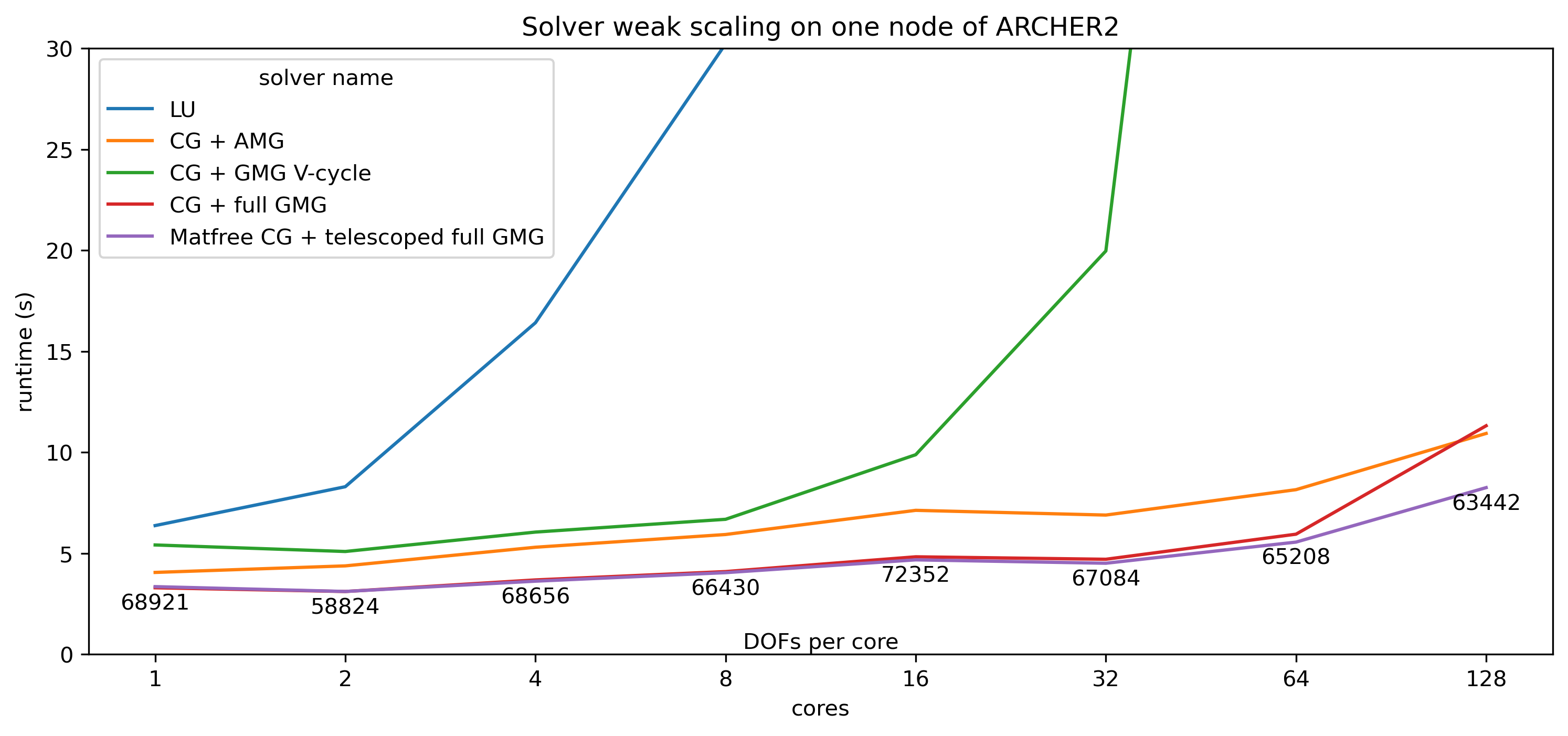
We can measure the weak scaling performance of the solvers by increasing the size of the problem in line with the number of processors. This is done approximately in the plot below, the number of DOFs per core is displayed underneath each data point. For a solver that weak scales perfectly, when we use twice as many cores to solve a problem twice as large, the total runtime should be the same and the lines in the plot should be approximately constant.
In the weak scaling plot below, CG + GMG V-cycles weak scales for longer than the LU factorisation and CG + AMG does even better, but we also see that in this setup we can do even better with full GMG methods.
Geometric Multigrid
Using the multigrid hierarchy is possible to solve the Poisson problem using full multigrid sweeps (sometimes called F-cycles).
By carefully choosing the number of smoothing steps (mg_levels_ksp_max_it) the number of CG iterations can be minimised.
[8]:
u_h.assign(0)
fmg = {
    "snes_view": None,
    "ksp_type": "cg",
    "pc_type": "mg",
    "pc_mg_log": None,
    "pc_mg_type": "full",
    "mg_levels_ksp_type": "chebyshev",
    "mg_levels_ksp_max_it": 2,
    "mg_levels_pc_type": "jacobi",
    "mg_coarse_pc_type": "lu",
    "mg_coarse_pc_factor_mat_solver_type": "mumps"
}
run_solve(problem, fmg)
parprint("Error   :", errornorm(truth, u_h))
SNES Object: (firedrake_3_) 1 MPI process
  type: ksponly
  maximum iterations=50, maximum function evaluations=10000
  tolerances: relative=1e-08, absolute=1e-50, solution=1e-08
  total number of linear solver iterations=5
  total number of function evaluations=1
  norm schedule ALWAYS
  KSP Object: (firedrake_3_) 1 MPI process
    type: cg
    maximum iterations=10000, initial guess is zero
    tolerances: relative=1e-07, absolute=1e-50, divergence=10000.
    left preconditioning
    using PRECONDITIONED norm type for convergence test
  PC Object: (firedrake_3_) 1 MPI process
    type: mg
      type is FULL, levels=3 cycles=v
        Not using Galerkin computed coarse grid matrices
    Coarse grid solver -- level 0 -------------------------------
      KSP Object: (firedrake_3_mg_coarse_) 1 MPI process
        type: preonly
        maximum iterations=10000, initial guess is zero
        tolerances: relative=1e-05, absolute=1e-50, divergence=10000.
        left preconditioning
        not checking for convergence
      PC Object: (firedrake_3_mg_coarse_) 1 MPI process
        type: lu
          out-of-place factorization
          tolerance for zero pivot 2.22045e-14
          using diagonal shift on blocks to prevent zero pivot [INBLOCKS]
          matrix ordering: external
          factor fill ratio given 0., needed 0.            Factored matrix:
              Mat Object: (firedrake_3_mg_coarse_) 1 MPI process
                type: mumps
                rows=4913, cols=4913
                package used to perform factorization: mumps
                total: nonzeros=1924469, allocated nonzeros=1924469
                  MUMPS run parameters:
                    Use -firedrake_3_mg_coarse_ksp_view ::ascii_info_detail to display information for all processes
                    RINFOG(1) (global estimated flops for the elimination after analysis): 6.40341e+08
                    RINFOG(2) (global estimated flops for the assembly after factorization): 2.37741e+06
                    RINFOG(3) (global estimated flops for the elimination after factorization): 6.40341e+08
                    (RINFOG(12) RINFOG(13))*2^INFOG(34) (determinant): (0.,0.)*(2^0)                    INFOG(3) (estimated real workspace for factors on all processors after analysis): 1924469
                    INFOG(4) (estimated integer workspace for factors on all processors after analysis): 44942
                    INFOG(5) (estimated maximum front size in the complete tree): 663
                    INFOG(6) (number of nodes in the complete tree): 194
                    INFOG(7) (ordering option effectively used after analysis): 2
                    INFOG(8) (structural symmetry in percent of the permuted matrix after analysis): 100
                    INFOG(9) (total real/complex workspace to store the matrix factors after factorization): 1924469
                    INFOG(10) (total integer space store the matrix factors after factorization): 44942
                    INFOG(11) (order of largest frontal matrix after factorization): 663
                    INFOG(12) (number of off-diagonal pivots): 0
                    INFOG(13) (number of delayed pivots after factorization): 0
                    INFOG(14) (number of memory compress after factorization): 0
                    INFOG(15) (number of steps of iterative refinement after solution): 0
                    INFOG(16) (estimated size (in MB) of all MUMPS internal data for factorization after analysis: value on the most memory consuming processor): 22
                    INFOG(17) (estimated size of all MUMPS internal data for factorization after analysis: sum over all processors): 22
                    INFOG(18) (size of all MUMPS internal data allocated during factorization: value on the most memory consuming processor): 22
                    INFOG(19) (size of all MUMPS internal data allocated during factorization: sum over all processors): 22
                    INFOG(20) (estimated number of entries in the factors): 1924469
                    INFOG(21) (size in MB of memory effectively used during factorization - value on the most memory consuming processor): 19
                    INFOG(22) (size in MB of memory effectively used during factorization - sum over all processors): 19
                    INFOG(23) (after analysis: value of ICNTL(6) effectively used): 0
                    INFOG(24) (after analysis: value of ICNTL(12) effectively used): 1
                    INFOG(25) (after factorization: number of pivots modified by static pivoting): 0
                    INFOG(28) (after factorization: number of null pivots encountered): 0
                    INFOG(29) (after factorization: effective number of entries in the factors (sum over all processors)): 1924469
                    INFOG(30, 31) (after solution: size in Mbytes of memory used during solution phase): 20, 20
                    INFOG(32) (after analysis: type of analysis done): 1
                    INFOG(33) (value used for ICNTL(8)): 7
                    INFOG(34) (exponent of the determinant if determinant is requested): 0
                    INFOG(35) (after factorization: number of entries taking into account BLR factor compression - sum over all processors): 1924469
                    INFOG(36) (after analysis: estimated size of all MUMPS internal data for running BLR in-core - value on the most memory consuming processor): 0
                    INFOG(37) (after analysis: estimated size of all MUMPS internal data for running BLR in-core - sum over all processors): 0
                    INFOG(38) (after analysis: estimated size of all MUMPS internal data for running BLR out-of-core - value on the most memory consuming processor): 0
                    INFOG(39) (after analysis: estimated size of all MUMPS internal data for running BLR out-of-core - sum over all processors): 0
        linear system matrix, which is also used to construct the preconditioner:
        Mat Object: (firedrake_3_mg_levels_0_) 1 MPI process
          type: seqaij
          rows=4913, cols=4913
          total: nonzeros=126785, allocated nonzeros=126785
          total number of mallocs used during MatSetValues calls=0
            not using I-node routines
    Down solver (pre-smoother) on level 1 -------------------------------
      KSP Object: (firedrake_3_mg_levels_1_) 1 MPI process
        type: chebyshev
          Chebyshev polynomial of first kind
          eigenvalue targets used: min 0.19855, max 2.18404
          eigenvalues estimated via gmres: min 0.0436521, max 1.9855
          eigenvalues estimated using gmres with transform: [0. 0.1; 0. 1.1]          KSP Object: (firedrake_3_mg_levels_1_esteig_) 1 MPI process
            type: gmres
              restart=30, using classical (unmodified) Gram-Schmidt orthogonalization with no iterative refinement
              happy breakdown tolerance=1e-30
            maximum iterations=10, initial guess is zero
            tolerances: relative=1e-12, absolute=1e-50, divergence=10000.
            left preconditioning
            using PRECONDITIONED norm type for convergence test
          estimating eigenvalues using a noisy random number generated right-hand side
        maximum iterations=2, nonzero initial guess
        tolerances: relative=1e-05, absolute=1e-50, divergence=10000.
        left preconditioning
        not checking for convergence
      PC Object: (firedrake_3_mg_levels_1_) 1 MPI process
        type: jacobi
          type DIAGONAL
        linear system matrix, which is also used to construct the preconditioner:
        Mat Object: (firedrake_3_mg_levels_1_) 1 MPI process
          type: seqaij
          rows=35937, cols=35937
          total: nonzeros=977793, allocated nonzeros=977793
          total number of mallocs used during MatSetValues calls=0
            not using I-node routines
    Up solver (post-smoother) same as down solver (pre-smoother)
    Down solver (pre-smoother) on level 2 -------------------------------
      KSP Object: (firedrake_3_mg_levels_2_) 1 MPI process
        type: chebyshev
          Chebyshev polynomial of first kind
          eigenvalue targets used: min 0.199079, max 2.18987
          eigenvalues estimated via gmres: min 0.0476982, max 1.99079
          eigenvalues estimated using gmres with transform: [0. 0.1; 0. 1.1]          KSP Object: (firedrake_3_mg_levels_2_esteig_) 1 MPI process
            type: gmres
              restart=30, using classical (unmodified) Gram-Schmidt orthogonalization with no iterative refinement
              happy breakdown tolerance=1e-30
            maximum iterations=10, initial guess is zero
            tolerances: relative=1e-12, absolute=1e-50, divergence=10000.
            left preconditioning
            using PRECONDITIONED norm type for convergence test
          estimating eigenvalues using a noisy random number generated right-hand side
        maximum iterations=2, nonzero initial guess
        tolerances: relative=1e-05, absolute=1e-50, divergence=10000.
        left preconditioning
        not checking for convergence
      PC Object: (firedrake_3_mg_levels_2_) 1 MPI process
        type: jacobi
          type DIAGONAL
        linear system matrix, which is also used to construct the preconditioner:
        Mat Object: (firedrake_3_) 1 MPI process
          type: seqaij
          rows=274625, cols=274625
          total: nonzeros=7678721, allocated nonzeros=7678721
          total number of mallocs used during MatSetValues calls=0
            not using I-node routines
    Up solver (post-smoother) same as down solver (pre-smoother)
    linear system matrix, which is also used to construct the preconditioner:
    Mat Object: (firedrake_3_) 1 MPI process
      type: seqaij
      rows=274625, cols=274625
      total: nonzeros=7678721, allocated nonzeros=7678721
      total number of mallocs used during MatSetValues calls=0
        not using I-node routines
Runtime : 2.817049741744995
Error   : 1.7378845762002274e-05
Using full GMG gives a significant speed up over using multigrid V-cycles as a preconditioner.
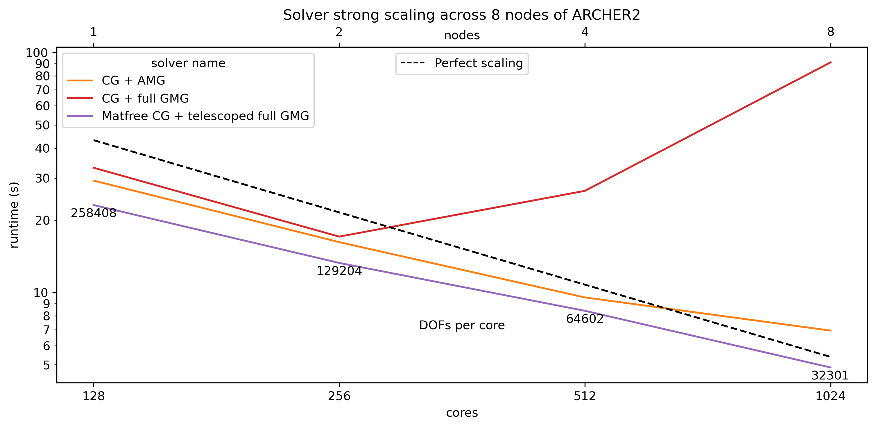
We can measure the strong scaling performance of the multigrid by choosing a large enough problem and seeing how long it takes to solve on different numbers of processes. In the plot below, the number of DOFs per core is displayed underneath each data point. For a solver that strong scales perfectly, when we use twice as many cores to solve the same size problem, the total runtime should be halved. This perfect scaling is plotted as a dashed line for comparison.
The figure below shows what happens when we use this multigrid solver for a large problem. For this test we set Nx = 10 and Nref = 4 to make a problem with 33 076 161 DOFs and solve over multiple nodes.
The full multigrid solver strong scales poorly beyond 2 nodes, the reason for this poor scaling is that the solver spends most of its time performing communication solving the problem on the coarse grid in a distributed manner. CG + AMG scales much better, but isn’t as fast as using telescoping, which we discuss in the next section. Designing a solver that is both fast and scalable for a given problem is often very challenging.
Matrix free and telescoping
In this section we show a final variation of the full multigrid solver above, which has advantages for larger problems and on HPC architectures.
One key advantage of using geometric multigrid over algebraic multigrid is the ability to use matrix free methods. These methods never assemble the full finite element matrix, which for large problems gives a significant reduction in memory usage. More information on matrix free methods in Firedrake can be found in the documentation. On the coarsest mesh of the multigrid hierarchy we can use the firedrake.AssembledPC to assemble the
finite element matrix, which allows us to use a direct solver.
The final set of solver options also deals with very large problems spread over multiple compute nodes. For a problem with a large multigrid hierarchy, the coarse grid problem is often so small that when it is solved over multiple nodes, the coarse solve spends all its time performing communication, which is slow.
The solution is to let each node solve a local copy of the coarse grid problem, which avoids this communication. This functionality is enabled using the telescope preconditioner alongside the assembled preconditioner, as shown below:
[9]:
u_h.assign(0)
telescope_factor = 1 # Set to number of nodes!
fmg_matfree_telescope = {
    "snes_view": None,
    "mat_type": "matfree",
    "ksp_type": "cg",
    "pc_type": "mg",
    "pc_mg_log": None,
    "pc_mg_type": "full",
    "mg_levels_ksp_type": "chebyshev",
    "mg_levels_ksp_max_it": 2,
    "mg_levels_pc_type": "jacobi",
    "mg_coarse": {
        "mat_type": "aij",
        "pc_type": "telescope",
        "pc_telescope_reduction_factor": telescope_factor,
        "pc_telescope_subcomm_type": "contiguous",
        "telescope_pc_type": "lu",
        "telescope_pc_factor_mat_solver_type": "mumps"
    }
}
run_solve(problem, fmg_matfree_telescope)
parprint("Error   :", errornorm(truth, u_h))
SNES Object: (firedrake_4_) 1 MPI process
  type: ksponly
  maximum iterations=50, maximum function evaluations=10000
  tolerances: relative=1e-08, absolute=1e-50, solution=1e-08
  total number of linear solver iterations=5
  total number of function evaluations=1
  norm schedule ALWAYS
  KSP Object: (firedrake_4_) 1 MPI process
    type: cg
    maximum iterations=10000, initial guess is zero
    tolerances: relative=1e-07, absolute=1e-50, divergence=10000.
    left preconditioning
    using PRECONDITIONED norm type for convergence test
  PC Object: (firedrake_4_) 1 MPI process
    type: mg
      type is FULL, levels=3 cycles=v
        Not using Galerkin computed coarse grid matrices
    Coarse grid solver -- level 0 -------------------------------
      KSP Object: (firedrake_4_mg_coarse_) 1 MPI process
        type: preonly
        maximum iterations=10000, initial guess is zero
        tolerances: relative=1e-05, absolute=1e-50, divergence=10000.
        left preconditioning
        not checking for convergence
      PC Object: (firedrake_4_mg_coarse_) 1 MPI process
        type: telescope
          PETSc subcomm: parent comm size reduction factor = 1
          PETSc subcomm: parent_size = 1 , subcomm_size = 1
          PETSc subcomm type = CONTIGUOUS
          setup type: default
          Parent DM object:         type = shell;
          Sub DM object: NULL
          KSP Object: (firedrake_4_mg_coarse_telescope_) 1 MPI process
            type: preonly
            maximum iterations=10000, initial guess is zero
            tolerances: relative=1e-05, absolute=1e-50, divergence=10000.
            left preconditioning
            not checking for convergence
          PC Object: (firedrake_4_mg_coarse_telescope_) 1 MPI process
            type: lu
              out-of-place factorization
              tolerance for zero pivot 2.22045e-14
              matrix ordering: external
              factor fill ratio given 0., needed 0.
                Factored matrix:
                  Mat Object: (firedrake_4_mg_coarse_telescope_) 1 MPI process
                    type: mumps
                    rows=4913, cols=4913
                    package used to perform factorization: mumps
                    total: nonzeros=1924469, allocated nonzeros=1924469
                      MUMPS run parameters:
                        Use -firedrake_4_mg_coarse_telescope_ksp_view ::ascii_info_detail to display information for all processes
                        RINFOG(1) (global estimated flops for the elimination after analysis): 6.40341e+08
                        RINFOG(2) (global estimated flops for the assembly after factorization): 2.37741e+06
                        RINFOG(3) (global estimated flops for the elimination after factorization): 6.40341e+08
                        (RINFOG(12) RINFOG(13))*2^INFOG(34) (determinant): (0.,0.)*(2^0)
                        INFOG(3) (estimated real workspace for factors on all processors after analysis): 1924469
                        INFOG(4) (estimated integer workspace for factors on all processors after analysis): 44942
                        INFOG(5) (estimated maximum front size in the complete tree): 663
                        INFOG(6) (number of nodes in the complete tree): 194
                        INFOG(7) (ordering option effectively used after analysis): 2
                        INFOG(8) (structural symmetry in percent of the permuted matrix after analysis): 100
                        INFOG(9) (total real/complex workspace to store the matrix factors after factorization): 1924469
                        INFOG(10) (total integer space store the matrix factors after factorization): 44942
                        INFOG(11) (order of largest frontal matrix after factorization): 663
                        INFOG(12) (number of off-diagonal pivots): 0
                        INFOG(13) (number of delayed pivots after factorization): 0
                        INFOG(14) (number of memory compress after factorization): 0
                        INFOG(15) (number of steps of iterative refinement after solution): 0
                        INFOG(16) (estimated size (in MB) of all MUMPS internal data for factorization after analysis: value on the most memory consuming processor): 22
                        INFOG(17) (estimated size of all MUMPS internal data for factorization after analysis: sum over all processors): 22
                        INFOG(18) (size of all MUMPS internal data allocated during factorization: value on the most memory consuming processor): 22
                        INFOG(19) (size of all MUMPS internal data allocated during factorization: sum over all processors): 22
                        INFOG(20) (estimated number of entries in the factors): 1924469
                        INFOG(21) (size in MB of memory effectively used during factorization - value on the most memory consuming processor): 19
                        INFOG(22) (size in MB of memory effectively used during factorization - sum over all processors): 19
                        INFOG(23) (after analysis: value of ICNTL(6) effectively used): 0
                        INFOG(24) (after analysis: value of ICNTL(12) effectively used): 1
                        INFOG(25) (after factorization: number of pivots modified by static pivoting): 0
                        INFOG(28) (after factorization: number of null pivots encountered): 0
                        INFOG(29) (after factorization: effective number of entries in the factors (sum over all processors)): 1924469
                        INFOG(30, 31) (after solution: size in Mbytes of memory used during solution phase): 20, 20
                        INFOG(32) (after analysis: type of analysis done): 1
                        INFOG(33) (value used for ICNTL(8)): 7
                        INFOG(34) (exponent of the determinant if determinant is requested): 0
                        INFOG(35) (after factorization: number of entries taking into account BLR factor compression - sum over all processors): 1924469
                        INFOG(36) (after analysis: estimated size of all MUMPS internal data for running BLR in-core - value on the most memory consuming processor): 0
                        INFOG(37) (after analysis: estimated size of all MUMPS internal data for running BLR in-core - sum over all processors): 0
                        INFOG(38) (after analysis: estimated size of all MUMPS internal data for running BLR out-of-core - value on the most memory consuming processor): 0
                        INFOG(39) (after analysis: estimated size of all MUMPS internal data for running BLR out-of-core - sum over all processors): 0
            linear system matrix, which is also used to construct the preconditioner:
            Mat Object: 1 MPI process
              type: seqaij
              rows=4913, cols=4913
              total: nonzeros=126785, allocated nonzeros=126785
              total number of mallocs used during MatSetValues calls=0
                not using I-node routines
        linear system matrix, which is also used to construct the preconditioner:
        Mat Object: (firedrake_4_mg_levels_0_) 1 MPI process
          type: seqaij
          rows=4913, cols=4913
          total: nonzeros=126785, allocated nonzeros=126785
          total number of mallocs used during MatSetValues calls=0
            not using I-node routines
    Down solver (pre-smoother) on level 1 -------------------------------
      KSP Object: (firedrake_4_mg_levels_1_) 1 MPI process
        type: chebyshev
          Chebyshev polynomial of first kind
          eigenvalue targets used: min 0.19855, max 2.18404
          eigenvalues estimated via gmres: min 0.0436521, max 1.9855
          eigenvalues estimated using gmres with transform: [0. 0.1; 0. 1.1]          KSP Object: (firedrake_4_mg_levels_1_esteig_) 1 MPI process
            type: gmres
              restart=30, using classical (unmodified) Gram-Schmidt orthogonalization with no iterative refinement
              happy breakdown tolerance=1e-30
            maximum iterations=10, initial guess is zero
            tolerances: relative=1e-12, absolute=1e-50, divergence=10000.
            left preconditioning
            using PRECONDITIONED norm type for convergence test
          estimating eigenvalues using a noisy random number generated right-hand side
        maximum iterations=2, nonzero initial guess
        tolerances: relative=1e-05, absolute=1e-50, divergence=10000.
        left preconditioning
        not checking for convergence
      PC Object: (firedrake_4_mg_levels_1_) 1 MPI process
        type: jacobi
          type DIAGONAL
        linear system matrix, which is also used to construct the preconditioner:
        Mat Object: (firedrake_4_mg_levels_1_) 1 MPI process
          type: python
          rows=35937, cols=35937
              Python: firedrake.matrix_free.operators.ImplicitMatrixContext
            Firedrake matrix-free operator ImplicitMatrixContext
    Up solver (post-smoother) same as down solver (pre-smoother)
    Down solver (pre-smoother) on level 2 -------------------------------
      KSP Object: (firedrake_4_mg_levels_2_) 1 MPI process
        type: chebyshev
          Chebyshev polynomial of first kind
          eigenvalue targets used: min 0.199079, max 2.18987
          eigenvalues estimated via gmres: min 0.0476982, max 1.99079
          eigenvalues estimated using gmres with transform: [0. 0.1; 0. 1.1]          KSP Object: (firedrake_4_mg_levels_2_esteig_) 1 MPI process
            type: gmres
              restart=30, using classical (unmodified) Gram-Schmidt orthogonalization with no iterative refinement
              happy breakdown tolerance=1e-30
            maximum iterations=10, initial guess is zero
            tolerances: relative=1e-12, absolute=1e-50, divergence=10000.
            left preconditioning
            using PRECONDITIONED norm type for convergence test
          estimating eigenvalues using a noisy random number generated right-hand side
        maximum iterations=2, nonzero initial guess
        tolerances: relative=1e-05, absolute=1e-50, divergence=10000.
        left preconditioning
        not checking for convergence
      PC Object: (firedrake_4_mg_levels_2_) 1 MPI process
        type: jacobi
          type DIAGONAL
        linear system matrix, which is also used to construct the preconditioner:
        Mat Object: (firedrake_4_) 1 MPI process
          type: python
          rows=274625, cols=274625
              Python: firedrake.matrix_free.operators.ImplicitMatrixContext
            Firedrake matrix-free operator ImplicitMatrixContext
    Up solver (post-smoother) same as down solver (pre-smoother)
    linear system matrix, which is also used to construct the preconditioner:
    Mat Object: (firedrake_4_) 1 MPI process
      type: python
      rows=274625, cols=274625
          Python: firedrake.matrix_free.operators.ImplicitMatrixContext
        Firedrake matrix-free operator ImplicitMatrixContext
Runtime : 3.150400161743164
Error   : 1.7378845761322788e-05
Running on HPC
To run these examples on HPC, the Firedrake code must be a Python script. Copy and paste these notebook cells into a text editor on the remote machine and save it as a Python script (extension .py).
The code must run through a job scheduler using another script. An example job script suitable for running on ARCHER2 is provided below.
To use this script change the account (-A) to your account, change the number of nodes (--node=) to the number of nodes you want to use and the time (-t) as appropriate, it is currently set to 10 minutes.
!/bin/bash
#SBATCH -p standard
#SBATCH -A account
#SBATCH -J firedrake
#SBATCH --nodes=1
#SBATCH --cpus-per-task=1
#SBATCH --qos=standard
#SBATCH -t 0:10:00

export VENV_NAME=firedrake_08_2021
export WORK=/work/e682/shared/firedrake_tarballs/firedrake_08_2021/
export FIREDRAKE_TEMP=firedrake_tmp
export LOCAL_BIN=$WORK

myScript="HPC_demo.py"

module load epcc-job-env

## Activate Firedrake venv (activate once on first node, extract once per node)
source $LOCAL_BIN/firedrake_activate.sh
srun --ntasks-per-node 1 $LOCAL_BIN/firedrake_activate.sh

## Run Firedrake script
srun --ntasks-per-node 128 $VIRTUAL_ENV/bin/python ${myScript}
If you named your jobscript jobscript.slm, then it can be submitted to the queue by running the following command on ARCHER2:
sbatch jobscript.slm
You can see your job’s progress through the queue using:
squeue -u $USER
If you need to cancel a job for any reason, you can pass your job ID number as an argument to the scancel command:
scancel 123456
Once your job has completed any output will be stored in files named slurm-123456.out and slurm-123456.err. The job ID 123456 is used as an example here, yours will be different each time you run a job.
Exercise
Perform a convergence study for the Poisson problem above, using degree 2 Lagrange elements. To do this, solve the problem on a range of different mesh sizes. The cell diameter on the finest mesh in a multigrid hierarchy is given by \(h = \frac{\sqrt{2}}{N}\), where \(N = N_x \times 2^{N_{ref}}\) is the number of cells along one edge of the cube on the finest grid.
Note: If you’re following along as part of a tutorial you will be assigned a single grid size and this exercise will be completed as a group.
Choose an appropriate number of multigrid levels (Nref) and coarse grid size (Nx) for each mesh size N. For this exercise we will repeatedly double \(N\) (to half the value of \(h\)), and measure the error for each solution. Use your answers to populate the table below:
N = |
8 |
16 |
32 |
64 |
128 |
256 |
512 |
|---|---|---|---|---|---|---|---|
Nx |
8 |
||||||
Nref |
2 |
Throughout the exercise we have already entered appropriate values into the table. These values correspond to the case presented in the notebook.
Calculate the number of DOFs for each problem size using the formula in the How big? section above. Use the total number of DOFs to work out how many processes would be appropriate for solving each problem size (try to pick a power of 2) and hence how many nodes you require for that simulation. Place all these values in the table:
N = |
8 |
16 |
32 |
64 |
128 |
256 |
512 |
|---|---|---|---|---|---|---|---|
DOFs |
274625 |
||||||
Processes |
4 |
||||||
Nodes |
1 |
For each problem size (or your given problem size if you are in a group) we will execute a Python script on the HPC to solve the Poisson problem.
Copy the cell containing the submission script in the Running on HPC above to your text editor on the HPC. Using your answer to (b), edit the lines #SBATCH --nodes=1 to the number of nodes you require for your problem size and the parameter --ntasks-per-node in the line:
srun --ntasks-per-node 128 $VIRTUAL_ENV/bin/python ${myScript}
to the number of processes you require. Save the file as jobscript.slm.
Next we must create a Firedrake script to run on HPC. If you are following as part of a tutorial a template will be provided, otherwise you can copy and paste code from cells in the notebook. Edit the values of Nx and Nref in the script to solve your selected problem size using your answer to (a). Ensure you save the files as HPC_demo.py
Finally, submit the job to the queue using the command sbatch jobscript.slm on the HPC command line and, once the job has run, check the output files current directory and fill in the error in the table below:
N = |
8 |
16 |
32 |
64 |
128 |
256 |
512 |
|---|---|---|---|---|---|---|---|
h |
0.044 |
||||||
Error |
1.74E-05 |
If you are performing the convergence study individually, continue editing the scripts to populate the rest of the table. Both the Python script and jobscript need to be changed to suit the problem size!
Plot the error against h and measure the rate of convergence using matplotlib. If you are completing this as part of a tutorial submit your results from (c) to the instructor and they will combine the results and plot the graph.
Hints:
You don’t need much compute power to solve small problems on coarse meshes, these will likely fit on one node.
Remember to make your job big enough for the number of processes that you run:
Each MPI rank must own at least one cell in the mesh.
Firedrake performs better when there are more than 50000 DOFs per rank.