
Steady Boussinesq problem with integral constraints
This demo demonstrates how integral constraints can be imposed on a field that appears nonlinearly in the governing equations.
The demo was contributed by Aaron Baier-Reinio and Kars Knook.
We consider a nondimensionalised steady Boussinesq problem. The domain is \(\Omega \subset \mathbb{R}^2\) with boundary \(\Gamma\). The boundary value problem is:
The unknowns are the \(\mathbb{R}^2\)-valued velocity \(u\), scalar pressure \(p\) and temperature \(T\). The viscosity \(\mu(T)\) is assumed to be a known function of \(T\). Moreover \(\epsilon (u)\) denotes the symmetric gradient of \(u\) and \(f = (0, -1)^T\) the acceleration due to gravity. Inhomogeneous Neumann boundary conditions are imposed on \(\nabla T \cdot n\) through given data \(g\) which must satisfy a compatibility condition
Evidently the pressure \(p\) is only determined up to a constant, since it only appears in the problem through its gradient. This choice of constant is arbitrary and does not affect the model. The situation regarding the temperature \(T\) is, however, more subtle. For the sake of discussion let us first assume that \(\mu(T) = \mu_0\) is a constant that does not depend on \(T\). It is then clear that, just like the pressure, the temperature \(T\) is undetermined up to a constant. We shall pin this down by enforcing that the mean of \(T\) is a user-supplied constant \(T_0\),
The Boussinesq approximation assumes that density varies linearly with temperature. Hence, this constraint can be viewed as an indirect imposition on the total mass of fluid in \(\Omega\).
Now suppose that \(\mu(T)\) does depend on \(T\). For simplicity we use a basic power law \(\mu(T) = 10^{-4} \cdot T^{1/2}\) but emphasise that the precise functional form of \(\mu(T)\) is unimportant to this demo. We must still impose the integral constraint on \(T\) to obtain a unique solution, but the value of \(T_0\) now affects the model in a non-trivial way since \(\mu(T)\) and \(T\) are coupled (c.f. the figures at the bottom of the demo). In particular, this is not a “trivial” situation like the incompressible Stokes problem where the discretised Jacobians have a nullspace corresponding to the constant pressures. Instead, we have an integral constraint on \(T\) even though the discretised Jacobians do not have a nullspace corresponding to the constant temperatures.
We build the mesh using netgen, choosing a trapezoidal geometry to prevent hydrostatic equilibrium and allow for a non-trivial velocity solution.
from firedrake import *
import netgen.occ as ngocc

wp = ngocc.WorkPlane()
wp.MoveTo(0, 0)
wp.LineTo(2, 0)
wp.LineTo(2, 1)
wp.LineTo(0, 2)
wp.LineTo(0, 0)

shape = wp.Face()
shape.edges.Min(ngocc.X).name = "left"
shape.edges.Max(ngocc.X).name = "right"

ngmesh = ngocc.OCCGeometry(shape, dim=2).GenerateMesh(maxh=0.1)

left_id = [i+1 for i, name in enumerate(ngmesh.GetRegionNames(dim=1)) if name == "left"]
right_id = [i+1 for i, name in enumerate(ngmesh.GetRegionNames(dim=1)) if name == "right"]

mesh = Mesh(ngmesh)
x, y = SpatialCoordinate(mesh)
Next we set up the discrete function spaces. We use lowest-order Taylor–Hood elements for the velocity and pressure, and continuous piecewise-linear elements for the temperature. We introduce a Lagrange multiplier to enforce the integral constraint on \(T\):
U = VectorFunctionSpace(mesh, "CG", degree=2)
V = FunctionSpace(mesh, "CG", degree=1)
W = FunctionSpace(mesh, "CG", degree=1)
R = FunctionSpace(mesh, "R", 0)

Z = U * V * W * R
The trial and test functions are:
z = Function(Z)
(u, p, T_aux, l) = split(z)
(v, q, w, s) = split(TestFunction(Z))

T = T_aux + l
The test Lagrange multiplier s will allow us to impose the integral constraint on the temperature.
We use the trial Lagrange multiplier l by decomposing the discretised temperature field T
as T = T_aux + l where T_aux is the trial function from W.
The value of l will then be determined by the integral constraint on T.
The remaining problem data to be specified is the Neumann data, viscosity, acceleration due to gravity and \(T_0\). For the Neumann data we choose a parabolic profile on the left and right edges, and zero data on the top and bottom.
g_left = y*(y-2)                # Neumann data on the left
g_right = -8*y*(y-1)            # Neumann data on the right
mu = (1e-4) * T ** (1/2)        # Viscosity
f = as_vector([0, -1])          # Acceleration due to gravity
T0 = Constant(1)                # Mean of the temperature
The nonlinear form for the problem is:
F = (mu * inner(sym(grad(u)), sym(grad(v))) * dx    # Viscous terms
 - inner(p, div(v)) * dx                            # Pressure gradient
 - inner(f, T*v) * dx                               # Buoyancy term
 - inner(div(u), q) * dx                            # Incompressibility constraint
 + inner(dot(u, grad(T)), w) * dx                   # Temperature advection term
 + inner(grad(T), grad(w)) * dx                     # Temperature diffusion term
 - inner(g_left, w) * ds(tuple(left_id))            # Weakly imposed Neumann BC terms
 - inner(g_right, w) * ds(tuple(right_id))          # Weakly imposed Neumann BC terms
 + inner(T - T0, s) * dx                            # Integral constraint on T
 )
and the (strongly enforced) Dirichlet boundary conditions on \(u\) are enforced by:
bc_u = DirichletBC(Z.sub(0), 0, "on_boundary")
At this point we could form and solve a NonlinearVariationalProblem
using F and bc_u. However, the resultant problem has a nullspace of
dimension 2, corresponding to (i) shifting \(p\) by a constant \(C_1\)
and (ii) shifting \(l\) by a constant \(C_2\) while simultaneuosly shifting
\(T_{\textrm{aux}}\) by \(-C_2\).
One way of dealing with nullspaces in Firedrake is to pass a nullspace and
transpose_nullspace to NonlinearVariationalSolver. However, sometimes
this approach may not be practical. First, for nonlinear problems with Jacobians that
are not symmetric, it may not obvious what the transpose_nullspace is. A second
reason is that, when using customised PETSc linear solvers, it may be desirable
to directly eliminate the nullspace from the assembled Jacobian matrix, since one
cannot always be sure that the linear solver at hand is correctly utilising the provided
nullspace and transpose_nullspace.
To directly eliminate the nullspace we introduce a class FixAtPointBC which
implements a boundary condition that fixes a field at a single point.
import functools

class FixAtPointBC(DirichletBC):
   r'''A special BC object for pinning a function at a point.

   :arg V: the :class:`.FunctionSpace` on which the boundary condition should be applied.
   :arg g: the boundary condition value.
   :arg bc_point: the point at which to pin the function.
       The location of the finite element DOF nearest to bc_point is actually used.
   '''
   def __init__(self, V, g, bc_point):
       super().__init__(V, g, bc_point)

   @functools.cached_property
   def nodes(self):
       V = self.function_space()

       point = [tuple(self.sub_domain)]
       vom = VertexOnlyMesh(V.mesh(), point)
       P0 = FunctionSpace(vom, "DG", 0)
       Fvom = Cofunction(P0.dual()).assign(1)

       # Take the basis function with the largest abs value at bc_point
       v = TestFunction(V)
       F = assemble(interpolate(inner(v, v), Fvom))
       with F.dat.vec as Fvec:
           max_index, _ = Fvec.max()
       nodes = V.dof_dset.lgmap.applyInverse([max_index])
       nodes = nodes[nodes >= 0]
       return nodes
We use this to fix the pressure and auxiliary temperature at the origin:
aux_bcs = [FixAtPointBC(Z.sub(1), 0, (0, 0)),
           FixAtPointBC(Z.sub(2), 0, as_vector([0, 0]))]
FixAtPointBC takes three arguments: the function space to fix, the value with which it
will be fixed, and the location at which to fix. Generally FixAtPointBC will not fix
the function at exactly the supplied point; it will fix it at the finite element DOF closest
to that point. By default CG elements have DOFs on all mesh vertices, so if the supplied
point if a mesh vertex then CG fields will be fixed at exactly the supplied point.
Warning
A FixAtPointBC does more than just fix the corresponding trial function
at the chosen DOF. It also ensures that the corresponding test function
(which is equal to one at that DOF and zero at all others)
will no longer be used in the discretised variational problem.
One must be sure that it is mathematically acceptable to do this.
In the present setting this is acceptable owing to the homogeneous Dirichlet
boundary conditions on \(u\) and compatibility condition \(\int_{\Gamma} g \ {\rm d} s = 0\)
on the Neumann data. The former ensures that the rows in the discretised Jacobian
corresponding to the incompressibility constraint are linearly dependent
(if there are \(M\) rows, only \(M-1\) of them are linearly independent, since
the boundary conditions on \(u\) ensure that
\(\int_{\Omega} \nabla \cdot u \ {\rm d} x = 0\) automatically).
Similarily the rows in the Jacobian corresponding to the temperature advection-diffusion
equation are linearly independent (again, if there are \(M\) rows,
only \(M-1\) of them are linearly independent).
The effect of FixAtPointBC will be to remove one of the rows corresponding
to the incompressibility constraint and one corresponding to the temperature advection-diffusion
equation. Which row ends up getting removed is determined by the location of bc_point,
but in the present setting removing a given row is mathematically equivalent to removing any one of the others.
One could envisage a more complicated scenario than the one in this demo, wherein the Neumann data
depends nonlinearly on some other problem unknowns, and it only satisfies the compatibility condition
approximately (e.g. up to some discretization error).
In this case one would have to be very careful when using FixAtPointBC –
although similar cautionary behaviour would also have to be taken if using
nullspace and transpose_nullspace instead.
Finally, we form and solve the nonlinear variational problem for \(T_0 \in \{1, 10, 100, 1000, 10000 \}\):
NLVP = NonlinearVariationalProblem(F, z, bcs=[bc_u]+aux_bcs)
NLVS = NonlinearVariationalSolver(NLVP)

(u, p, T_aux, l) = z.subfunctions
File = VTKFile(f"output/boussinesq.pvd")

for i in range(0, 5):
    T0.assign(10**(i))
    l.assign(Constant(T0))
    NLVS.solve()

    u_out = assemble(project(u, Z.sub(0)))
    p_out = assemble(project(p, Z.sub(1)))
    T_out = assemble(project(T, Z.sub(2)))

    u_out.rename("u")
    p_out.rename("p")
    T_out.rename("T")

    File.write(u_out, p_out, T_out, time=i)
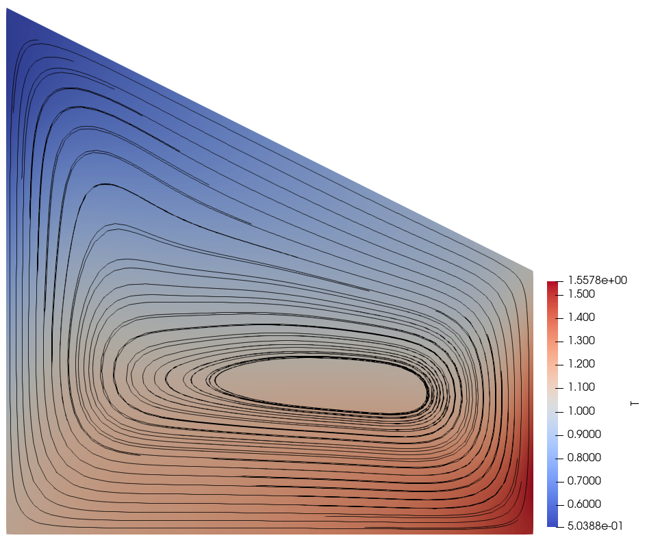
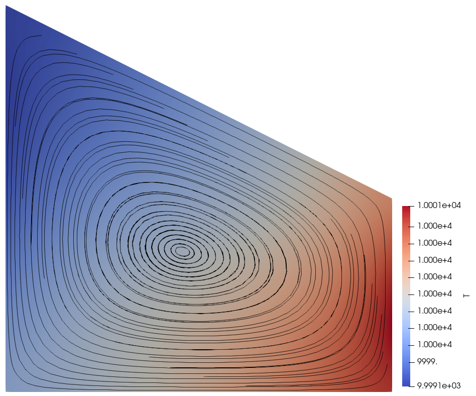
The temperature and stream lines for \(T_0=1\) and \(T_0=10000\) are displayed below on the left and right respectively.
|
|
A Python script version of this demo can be found here.