1D Vlasov-Poisson Equation

This tutorial was contributed by Colin Cotter and Werner Bauer.

A plasma is a continuum of moving particles with nonunique velocity at each point in space. In \(d\) dimensions, the plasma is described by a density \(f(x,v,t)\) where \(x\in \mathbb{R}^d\) are the physical coordinates and \(v \in \mathbb{R}^d\) are velocity coordinates. Hence, in \(d\) dimensions, a \(2d\) dimensional mesh is required. To deal with this curse of dimensionality, particle-in-cell methods are usually used. However, in 1 dimension, it is tractable to simulate the plasma on a 2 dimensional mesh.

The Vlasov equation models the (collisionless) conservation of plasma particles, according to

\[f_t + \nabla_{\vec{x}} \cdot (\vec{v}f) + \nabla_{\vec{v}} \cdot (\vec{a}f) = 0,\]

where

\[\nabla_{\vec{x}} = (\partial_{x_1},\ldots, \partial_{x_d}), \quad \nabla_{\vec{v}} = (\partial_{v_1},\ldots, \partial_{v_d}).\]

To close the system, we need a formula for the acceleration \(\vec{a}\). In the (single species) Vlasov-Poisson model, the acceleration is determined by the electrostatic force,

\[\vec{a} = -\frac{1}{m}\nabla\phi,\]

where \(m\) is the mass per plasma particle, and \(\phi\) is the electrostatic potential determined by the Poisson equation,

\[-\nabla^2\phi = q_0\int_{\mathbb{R}^d} f(\vec{x},\vec{v},t)\,\mathrm{d} v,\]

where \(q_0\) is the electric charge per plasma particle.

In this demo we specialise to \(d=1\), and the equations become

\[f_t + (fv)_x + (-f\phi_x/m)_v = 0, \quad -\phi_{xx} = q_0\int f(x,v,t)\,\mathrm{d} v,\]

with coordinates \((x,v)\in \mathbb{R}^2\). From now on we will relabel these coordinates \((x,v)\mapsto (x_1,x_2)\), obtaining the equivalent form,

\[f_t + \nabla\cdot(\vec{u}f) = 0, \quad \vec{u} = (v,-\phi_x/m), \quad -\phi_{x_1x_1} = q_0\int f(x_1,x_2,t)\,\mathrm{d} x_2,\]

where \(\nabla=(\partial_{x_1},\partial_{x_2})\). From now on we will choose units such that \(q_0,m\) are absorbed into the definition of \(f\).

To proceed, we need to develop variational formulations of these equations.

For the density we will use a discontinuous Galerkin formulation, and the continuity equation becomes

\[\begin{split}\int_\Omega \! q \frac{\partial f}{\partial t} \, \mathrm{d} x &= \int_\Omega \! f \nabla \cdot (q \vec{u}) \, \mathrm{d} x\\ &\quad- \int_{\Gamma_\mathrm{int}} \! \widetilde{f}(q_+ \vec{u} \cdot \vec{n}_+ + q_- \vec{u} \cdot \vec{n}_-) \, \mathrm{d} S\\ &\quad- \int_{\Gamma_I} q f_\mathrm{in} \vec{u} \cdot \vec{n} \, \mathrm{d} s\\ &\quad- \int_{\Gamma_O} q f \vec{u} \cdot \vec{n} \, \mathrm{d} s \qquad \forall q \in V,\end{split}\]

where \(\Omega\) is the computational domain in \((x,v)\) space, \(V\) is the discontinuous finite element space, \(\Gamma_\mathrm{int}\) is the set of interior cell edges, \(\Gamma_I\) is the inlet part of exterior boundary where \(\vec{u}\cdot\vec{n}<0\), \(\Gamma_O\) is the outlet part of exterior boundary where \(\vec{u}\cdot\vec{n}>0\), \(n\) is the normal to each edge, \(\tilde{f}\) is the upwind value of \(f\), and \(f_{\mathrm{in}}\) is the inflow boundary value for \(f\). See the Discontinuous Galerkin advection demo for more details. The unapproximated problem should have \(-\infty < x_2 < \infty\), i.e. unbounded velocities, but we approximate the problem by solving in the domain \(\Omega=I_1\times [-H/2, H/2]\), where \(I\) is some chosen interval in the spatial dimension.

For the Poisson equation, we will use a regular Galerkin formulation. The difficulty in the formulation is the integral over \(x_2\). We deal with this by considering a space \(\bar{W}\) which is restricted to functions that are constant in the vertical. Multiplying by a test function \(\psi\in \bar{W}\) and integrating by parts gives

\[\int \psi_{x_1}\phi_{x_1}\, \mathrm{d} x_1 = \int \int f(x_1,x_2,t) \psi\, \mathrm{d} x_1\,\mathrm{d} x_2, \quad \forall \psi \in \bar{W}.\]

Since the left hand side integrand is independent of \(v=x_2\), we can integrate over \(x_2\) and divide by \(H\), to obtain

\[\int_\Omega \psi_{x_1}\phi_{x_1}/H\, \mathrm{d} x = \int f \psi\, \mathrm{d} x, \quad \forall \psi \in \bar{W},\]

which is now in a form which we can implement easily in Firedrake. One final issue is that this problem only has a solution up to an additive constant, so we further restrict \(\phi \in \mathring{\bar{W}}\), where

\[\mathring{\bar{W}} = \{ w\in \bar{W}: \bar{w}=0\},\]

where here the bar indicates a spatial average,

\[\bar{w} = \frac{\int_{\Omega} w\, \mathrm{d} x}{\int_{\Omega} 1 \mathrm{d} x}.\]

Then we seek the solution of

\[\int_\Omega \psi_{x_1}\phi_{x_1}\,\mathrm{d} x = \int H(f-\bar{f}) \psi\, \mathrm{d} x, \quad \forall \psi \in \mathring{\bar{W}}.\]

To discretise in time, we will use an SSPRK3 time discretisation, similar to the DG advection demo. At each Runge-Kutta stage, we must solve for the electrostatic potential, and then use it to compute \(\vec{u}\), in order to compute \(\partial f/\partial t\).

As usual, to implement this problem, we start by importing the Firedrake namespace.

from firedrake import *

We build the mesh by constructing a 1D mesh, which will be extruded in the vertical. Here we will use periodic boundary conditions in the \(x_1\) direction,

ncells = 50
L = 8*pi
base_mesh = PeriodicIntervalMesh(ncells, L)

The mesh is then extruded upwards in the “velocity” direction.

H = 10.0
nlayers = 50
mesh = ExtrudedMesh(base_mesh, layers=nlayers, layer_height=H/nlayers)

We want to have \(v=0\) in the middle of the domain, so that we can have negative and positive velocities. This requires to edit the coordinate field.

x, v = SpatialCoordinate(mesh)
mesh.coordinates.interpolate(as_vector([x, v-H/2]))

Now we build a discontinuous finite element space for the density,

V = FunctionSpace(mesh, 'DQ', 1)

and a continuous finite element space for the electostatic potential. The space is continuous in the horizontal and constant in the vertical, specified through the vfamily.

Wbar = FunctionSpace(mesh, 'CG', 1, vfamily='R', vdegree=0)

We create a Function to store the solution at the current time, and then set its initial condition,

\[f(x,v,0) = \frac{1}{\sqrt{2\pi}}v^2\exp(-v^2/2)(1+ A\cos(kx)), \quad A=0.05, \quad k=0.5.\]

fn = Function(V, name="density")
A = Constant(0.05)
k = Constant(0.5)
fn.interpolate(v**2*exp(-v**2/2)*(1 + A*cos(k*x))/(2*pi)**0.5)

We will need the (conserved) average \(\bar{f}\) for the Poisson equation.

One = Function(V).assign(1.0)
fbar = assemble(fn*dx)/assemble(One*dx)

We create a Function to store the electrostatic potential.

phi = Function(Wbar, name="potential")

The next task is to create the solver for the electrostatic potential, which will be called every timestep.

We create a Function to store the intermediate densities at each Runge-Kutta stage. The right hand side of the Poisson equation will be evaluated using this Function to obtain the potential at each stage. Defining this beforehand will enable us to reuse the solver.

fstar = Function(V)

Now we express the Poisson equation in UFL.

psi = TestFunction(Wbar)
dphi = TrialFunction(Wbar)
phi_eqn = dphi.dx(0)*psi.dx(0)*dx - H*(fstar-fbar)*psi*dx

To deal mathematically with the null space of the potential, we expressed the problem in \(\mathring{\bar{W}}\). Programmatically we will express the problem in \(\bar{W}\) and deal with the null space by defining a basis for the space of globally constant functions, which we will later pass to PETSc so the solver can remove it from the solution.

nullspace = VectorSpaceBasis(constant=True, comm=COMM_WORLD)

However, the null space also means that the assembled matrix of the Poisson problem will be singular, which will prevent us from using a direct solver. To deal with this, we will precondition the Poisson problem with a version shifted by \(\int_{\Omega}\phi\psi\mathrm{d}x\). The shifted problem is well-posed on \(\bar{W}\), so the assembled matrix will be non-singular and so solvable with direct methods.

shift_eqn = dphi.dx(0)*psi.dx(0)*dx + dphi*psi*dx

We use these to define a LinearVariationalProblem.

phi_problem = LinearVariationalProblem(lhs(phi_eqn), rhs(phi_eqn),
                                       phi, aP=shift_eqn)

Now we build the LinearVariationalSolver. The problem is preconditioned by the shifted operator which is solved using a direct solver, and we pass the nullspace of globally constant functions to the solver.

params = {
   'ksp_type': 'gmres',
   'pc_type': 'lu',
   'ksp_rtol': 1.0e-8,
   }
phi_solver = LinearVariationalSolver(phi_problem,
                                     nullspace=nullspace,
                                     solver_parameters=params)

Now we move onto the solver to compute \(\partial f/\partial t\). We define a symbolic \(\Delta t\) which we will update later.

dtc = Constant(0)

At each stage, the solver will take in the intermediate solution fstar and return the stage increment \(\Delta t\partial f/\partial t\) in df_out.

df_out = Function(V)

Now we express the equation in UFL, starting with the left hand side bilinear form

q = TestFunction(V)
u = as_vector([v, -phi.dx(0)])
n = FacetNormal(mesh)
un = 0.5*(dot(u, n) + abs(dot(u, n)))
df = TrialFunction(V)
df_a = q*df*dx

The problem is defined on an extruded mesh, so the interior facets are separated into horizontal and vertical ones.

dS = dS_h + dS_v

Now we build the right hand side linear form. A conditional operator is used to deal with the inflow and outflow parts of the exterior boundary. Due to the periodic boundary conditions in \(x_1\), the only exterior boundary is at the top and bottom of the domain, with measure ds_tb.

df_L = dtc*(div(u*q)*fstar*dx
   - (q('+') - q('-'))*(un('+')*fstar('+') - un('-')*fstar('-'))*dS
   - conditional(dot(u, n) > 0, q*dot(u, n)*fstar, 0.)*ds_tb
    )

We then use this to build a solver.

df_problem = LinearVariationalProblem(df_a, df_L, df_out)
df_solver = LinearVariationalSolver(df_problem)

We are getting close to the time loop. We set up some timestepping parameters.

T = 50.0 # maximum timestep
t = 0. # model time
ndump = 100 # frequency of file dumps
dumpn = 0 # dump counter
nsteps = 5000
dt = T/nsteps
dtc.assign(dt)

We set up some Functions to store Runge-Kutta stage variables.

f1 = Function(V)
f2 = Function(V)

We set up a VTKFile object to write output every ndump timesteps.

outfile = VTKFile("vlasov.pvd")

We want to output the initial condition, so need to solve for the electrostatic potential that corresponds to the initial density.

fstar.assign(fn)
phi_solver.solve()
outfile.write(fn, phi)
phi.assign(.0)

Now we start the timeloop using a lovely progress bar. Note that we have 5000 timesteps so this may take a few minutes to run:

for step in ProgressBar("Timestep").iter(range(nsteps)):

Each Runge-Kutta stage involves solving for \(\phi\) before solving for \(\partial f/\partial t\). Here is the first stage.

#
    fstar.assign(fn)
    phi_solver.solve()
    df_solver.solve()
    f1.assign(fn + df_out)

The second stage.

#
    fstar.assign(f1)
    phi_solver.solve()
    df_solver.solve()
    f2.assign(3*fn/4 + (f1 + df_out)/4)

The third stage.

#
    fstar.assign(f2)
    phi_solver.solve()
    df_solver.solve()
    fn.assign(fn/3 + 2*(f2 + df_out)/3)
    t += dt

Finally we output to the VTK file if it is time to do that.

#
    dumpn += 1
    if dumpn % ndump == 0:
        dumpn = 0
        outfile.write(fn, phi)

Images of the solution at shown below.

Solution at \(t = 0.\)

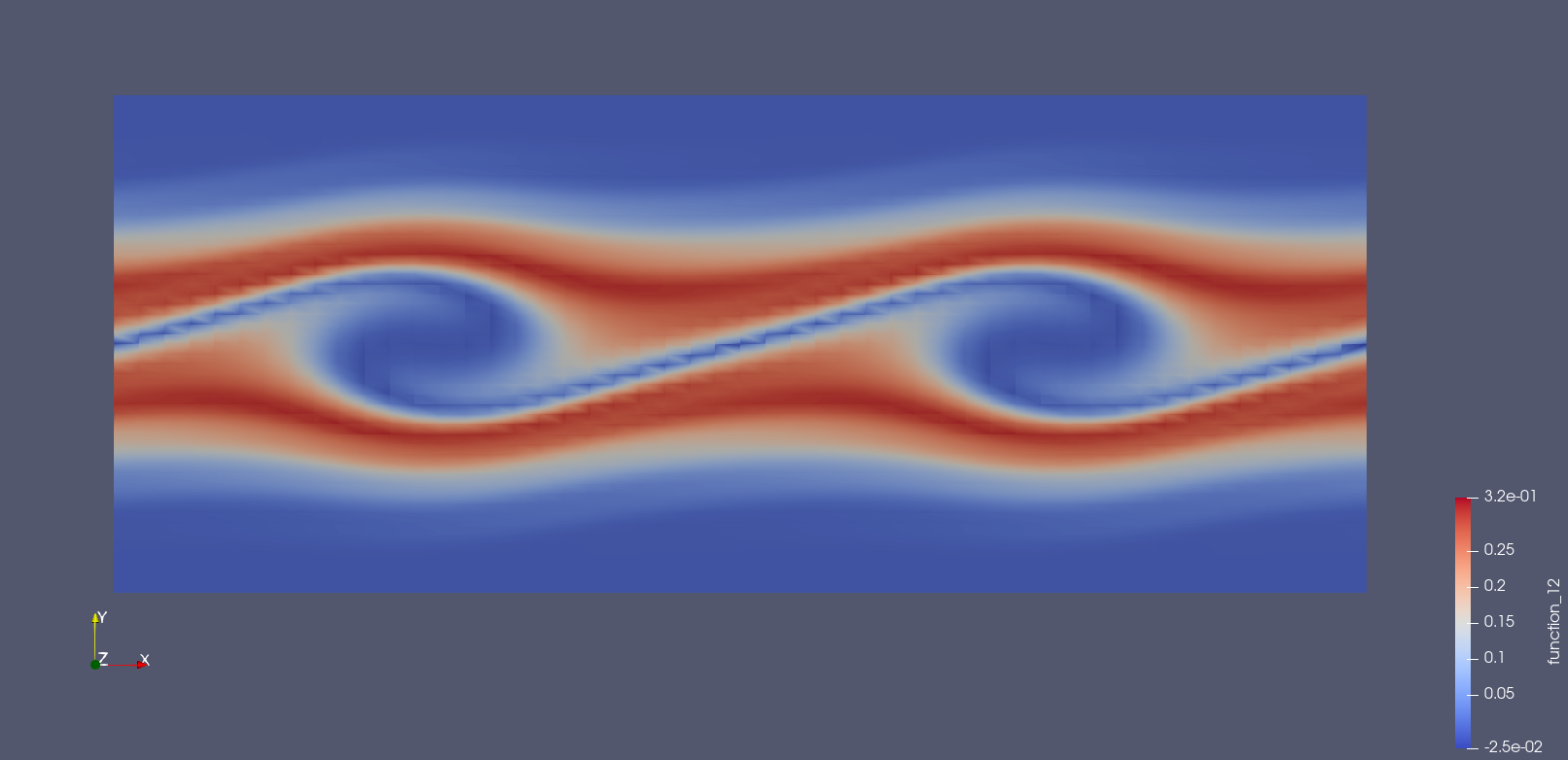
Solution at \(t = 15.\)

We also present solutions at double the resolution, by doubling the number of horizontal cells and the number of layers, halving the timestep (by doubling the number of steps), and doubling nsteps.

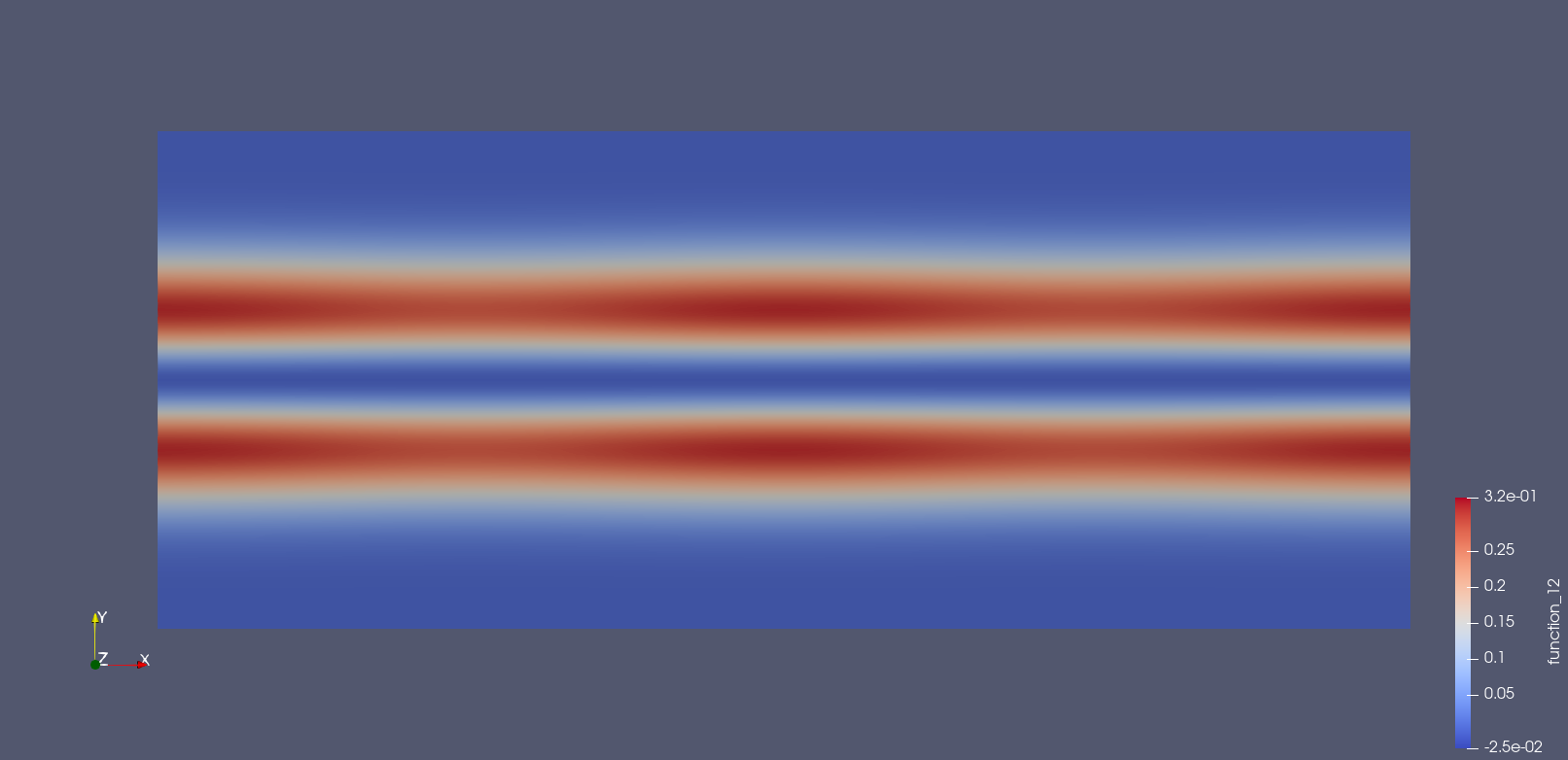
Solution at \(t = 0.\)

Solution at \(t = 15.\)

A Python script version of this demo can be found here.