
Multicomponent flow – microfluidic non-ideal mixing of hydrocarbons
We show how Firedrake can be used to simulate multicomponent flow, specifically the microfluidic non-ideal mixing of benzene and cyclohexane.
The demo was contributed by Aaron Baier-Reinio and Kars Knook.
Multicomponent fluids are those composed of two or more species. Solving the equations describing such fluids is challenging, because there are many variables to solve for, the equations are nonlinear, and because the system possesses subtle properties like the mass-average constraint and the mole fraction sum.
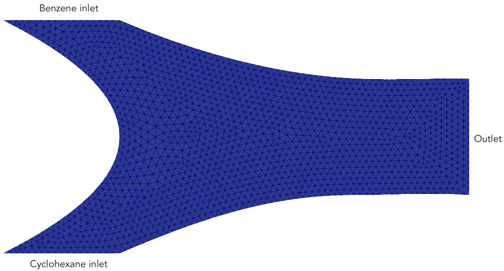
We consider a steady, isothermal, nonreacting mixture of benzene and cyclohexane in a two-dimensional microfluidic container \(\Omega \subset \mathbb{R}^2\). Pure benzene and cyclohexane flow in through opposing inlets on the left side of the container. The chemicals then mix in the center of the container and exit through an outlet on the right. We use netgen to build a curved mesh of order \(k=3\):
from firedrake import *
import netgen.occ as ngocc

# The polynomial order we will use for our curved mesh and finite element spaces
k = 3

# Specify the domain Omega (i.e. the microfluidic container's geometry)
wp = ngocc.WorkPlane()
wp.MoveTo(0, 1)
wp.Spline([ngocc.Pnt(1, 0), ngocc.Pnt(0, -1)])
wp.LineTo(1, -1)
wp.Spline([ngocc.Pnt(3, -0.5), ngocc.Pnt(4, -0.5)], tangents={ 1 : ngocc.gp_Vec2d(1, 0) })
wp.LineTo(4, 0.5)
wp.Spline([ngocc.Pnt(3, 0.5), ngocc.Pnt(1, 1)], tangents={ 0 : ngocc.gp_Vec2d(-1, 0) })
wp.LineTo(0, 1)

Omega = wp.Face()

# Label the inlets and outlet; the other walls are unlabelled
Omega.edges.Max(ngocc.Y).name = "inlet_1"
Omega.edges.Min(ngocc.Y).name = "inlet_2"
Omega.edges.Max(ngocc.X).name = "outlet"

# Smaller problem when running CI tests
import os
if os.getenv("FIREDRAKE_CI") == "1":
    maxh = 0.3
    k = 1
else:
    maxh = 0.055

# Construct the mesh
ngmesh = ngocc.OCCGeometry(Omega, dim=2).GenerateMesh(maxh=maxh)
mesh = Mesh(Mesh(ngmesh).curve_field(max(k, 2)))

# Get the IDs of the inlets, outlet and walls
inlet_1_id = tuple(i+1 for i, name in enumerate(ngmesh.GetRegionNames(dim=1)) if name == "inlet_1")
inlet_2_id = tuple(i+1 for i, name in enumerate(ngmesh.GetRegionNames(dim=1)) if name == "inlet_2")
outlet_id = tuple(i+1 for i, name in enumerate(ngmesh.GetRegionNames(dim=1)) if name == "outlet")
walls_ids = tuple(i+1 for i, name in enumerate(ngmesh.GetRegionNames(dim=1)) if name == "")

# Define the surface and volume measures using a fixed quadrature degree
deg_max = 3*k
ds = ds(mesh, degree=deg_max)
dx = dx(mesh, degree=deg_max)

# Define the spatial coordinates on the mesh
x_sc, y_sc = SpatialCoordinate(mesh)
The domain and mesh are visualised below.
To model the mixture we employ the Stokes–Onsager–Stefan–Maxwell (SOSM) partial differential equations and discretise with the method of [BRF26]. We use the material property values specified in [AFMVB25], wherein a similar benzene-cyclohexane simulation is considered. In what follows species 1 refers to benzene and species 2 to cyclohexane. We shall discretise the following unknowns:
\(J_1, J_2 \in \textrm{BDM}_k\) - species mass fluxes,
\(v \in [\textrm{CG}_k]^2\) - barycentric velocity,
\(\mu_1, \mu_2 \in \textrm{DG}_{k-1}\) - species chemical potentials,
\(p \in \textrm{CG}_{k-1}\) - pressure,
\(x_1, x_2 \in \textrm{DG}_{k-1}\) - species mole fractions,
\(\rho^{-1} \in \textrm{CG}_{k-1}\) - density reciprocal (i.e. specific volume).
The equations governing these unknowns are presented below. We first define the finite element spaces and trial/test functions:
# The finite element spaces
J_h = FunctionSpace(mesh, "BDM", k)                 # Species mass-flux space
V_h = VectorFunctionSpace(mesh, "CG", max(k, 2))    # Velocity space (minimum order is 2)
U_h = FunctionSpace(mesh, "DG", k - 1)              # Species chemical potential space
P_h = FunctionSpace(mesh, "CG", max(k - 1, 1))      # Pressure space (minimum order is 1)
X_h = FunctionSpace(mesh, "DG", k - 1)              # Species mole fraction space
R_h = FunctionSpace(mesh, "CG", max(k - 1, 1))      # Density reciprocal space (minimum order is 1)
L_h = FunctionSpace(mesh, "R", 0)                   # Lagrange multiplier space

# The mixed space
Z_h = J_h * J_h * V_h * U_h * U_h * P_h * X_h * X_h * R_h * L_h * L_h
PETSc.Sys.Print(f"Mesh has {mesh.num_cells()} cells, with {Z_h.dim()} finite element DOFs")

# The discrete solution
solution = Function(Z_h)
J_1, J_2, v, mu_aux_1, mu_aux_2, p, x_1, x_2, rho_inv, l_1, l_2 = split(solution)

# Lagrange multiplier trick for enforcing integral constraints
mu_1 = mu_aux_1 + l_1
mu_2 = mu_aux_2 + l_2

# The test functions
W_1, W_2, u, w_1, w_2, q, y_1, y_2, r, s_1, s_2 = TestFunctions(Z_h)
Note that we decompose the chemical potentials as \(\mu_i = \mu_{i, \textrm{aux}} + l_i\) where \(l_i\) are Lagrange multipliers. This will aid in enforcing integral constraints on the solution; see the steady Boussinesq demo for an explanation of the process.
Governing PDEs: SOSM Equations
Momentum transport is modelled using the steady compressible Stokes momentum equation for a Newtonian fluid,
Recall that \(v\) is the barycentric velocity and \(p\) the pressure. Moreover \(\epsilon (v)\) denotes the symmetric gradient of \(v\) while \(\eta, \zeta > 0\) are the shear and bulk viscosities respectively, \(d=2\) is the spatial dimension and \(\mathbb{I}\) the \(d \times d\) identity matrix. Despite the fact that we are considering compressible flow, we still need a constraint on \(\nabla \cdot v\) (as is the case for incompressible flow). However, we postpone the discussion of this constraint to the end of this section as it involves other quantities that we have not yet described.
We shall non-dimensionalise all of the unknowns in our discretisation. Hence we introduce a reference velocity \(v^{\textrm{ref}}\) whose value will be specified later on when we introduce boundary conditions. We also choose a reference length of \(L^{\textrm{ref}} = 2 \cdot 10^{-3}\) m. It is then natural to define the reference pressure as \(p^{\textrm{ref}} = \eta \cdot v^{\textrm{ref}} / L^{\textrm{ref}}\).
# The (dimensional) Stokes viscosities
eta = Constant(6e-4)            # Shear viscosity, Pa s
zeta = Constant(1e-7)           # Bulk viscosity, Pa s

# Non-dimensionalised Lamé parameter, dimensionless
lame_ND = (zeta / eta) - 1.0

# Reference quantities used for non-dimensionalisation
v_ref = Constant(0.0)           # Reference velocity (to be specified later), m / s
L_ref = Constant(2e-3)          # Reference length, m
p_ref = eta * v_ref / L_ref     # Reference pressure, Pa
The non-dimensionalised variational formulation of eq. 1 is then:
# The Stokes viscous terms
stokes_terms = 2.0 * inner(sym(grad(v)), sym(grad(u))) * dx
stokes_terms += lame_ND * inner(div(v), div(u)) * dx

# The Stokes pressure term
stokes_terms -= inner(p, div(u)) * dx
Let \(n \geq 2\) denote the number of chemical species. Hence \(n=2\) throughout this demo (benzene and cyclohexane). The continuity equation for the molar concentration \(c_i\) of species \(i \in \{1:n\}\) in the absence of chemical reactions is
where \(M_i > 0\) is the molar mass of species \(i\) and \(J_i\) its mass flux. As we are considering steady flow, the continuity equations simplify to
which are discretised as follows:
continuity_terms = (inner(div(J_1), w_1) + inner(div(J_2), w_2)) * dx
Next, we incorporate the volumetric equation of state, which models how the concentration of the mixture depends on temperature, pressure and composition. Composition of the mixture is described using mole fractions \(x_i := c_i / c_T\) where \(c_T = \sum_{j=1}^n c_j\) is the total concentration. Note that by definition \(\sum_{j=1}^n x_j = 1\), although at the discrete level this relation will only hold approximately. We assume that the mixture is quasi-incompressible in the sense that its partial molar volumes are constant; this is often a reasonable assumption for liquids. It follows that the volumetric equation of state is
where \(c_j^{\textrm{pure}}\) is the concentration of pure species \(j\). We use values for \(c_j^{\textrm{pure}}\) that are measured at room temperature \(T=298.15\) K and ambient pressure \(10^5\) Pa (note that we allow the pressure \(p\) to vary in this model but we assume that these variations do not alter \(c_j^{\textrm{pure}}\)). We will also make use of the total density of the mixture which is given by \(\rho = \sum_{j=1}^n M_j c_j\). To non-dimensionalise the concentrations and total density, we employ as reference values for these quantities their values when the mixture is equimolar:
# Constants for the pure species (at the ambient temperature and pressure)
M_1 = Constant(0.078)               # Molar mass of benzene, kg / mol
M_2 = Constant(0.084)               # Molar mass of cyclohexane, kg / mol
rho_pure_1 = Constant(876)          # Density of pure benzene, kg / m^3
rho_pure_2 = Constant(773)          # Density of pure cyclohexane, kg / m^3
c_pure_1 = rho_pure_1 / M_1         # Concentration of pure benzene, mol / m^3
c_pure_2 = rho_pure_2 / M_2         # Concentration of pure cyclohexane, mol / m^3

# Constants for the equimolar mixture
c_equi_tot = 1.0 / ((0.5 / c_pure_2) + (0.5 / c_pure_1))  # Total equimolar concentration, mol / m^3
c_equi_1 = 0.5 * c_equi_tot                     # Equimolar concentration of benzene, mol / m^3
c_equi_2 = 0.5 * c_equi_tot                     # Equimolar concentration of cyclohexane, mol / m^3
rho_equi = (M_1 * c_equi_1) + (M_2 * c_equi_2)  # Equimolar density, kg / m^3

# Reference concentration, density and molar mass
rho_ref = rho_equi                              # Reference density, kg / m^3
c_ref = c_equi_tot                              # Reference concentration, mol / m^3
M_ref = rho_ref / c_ref                         # Reference molar mass, kg / mol

# Non-dimensionalised molar masses
M_1_ND = M_1 / M_ref
M_2_ND = M_2 / M_ref
Our implementation of the non-dimensionalised volumetric equation of state eq. 3 is therefore:
# Volumetric equation of state, assuming constant partial molar volumes
def conc_relation(x_1, x_2):

    # Normalise the mole fractions before computing c_tot,
    # since they will only sum to one up to discretisation error
    x_1_nm = x_1 / (x_1 + x_2)
    x_2_nm = x_2 / (x_1 + x_2)

    # Compute c_tot and the species concentrations
    c_tot = 1.0 / ((x_1_nm * (c_ref / c_pure_1)) + (x_2_nm * (c_ref / c_pure_2)))
    c_1 = x_1_nm * c_tot
    c_2 = x_2_nm * c_tot

    return (c_tot, c_1, c_2)

c_tot, c_1, c_2 = conc_relation(x_1, x_2)
Moreover, to express that \(1 / \rho^{-1} = \rho = \sum_{j=1}^n M_j c_j\), we simply take the \(L^2\)-projection of this expression (in non-dimensionalised form):
rho_inv_terms = inner(1.0 / rho_inv, r) * dx
rho_inv_terms -= inner((M_1_ND * c_1) + (M_2_ND * c_2), r) * dx
Next, we must model how the free energy of the mixture depends on temperature, pressure and composition. This is accomplished by introducing the species chemical potentials \(\mu_i, \ i \in \{1 : n\}\), which are unknown scalar fields that describe the local chemical potential energy of the mixture. Thermodynamics requires that these satisfy
where \(g_i: \mathbb{R}^{n+2} \rightarrow \mathbb{R}\) are partial molar Gibbs functions. These functions are derived from partial derivatives of the Gibbs free energy of the mixture. It is natural to non-dimensionalise the chemical potentials using a reference value of \(\mu^{\textrm{ref}} = RT\) where \(R\) the is ideal gas constant and \(T\) the ambient temperature. In this demo we employ a Margules model [GP07] for the \(g_i\)’s, which in non-dimensionalised form, is implemented as follows:
RT = Constant(8.314 * 298.15)   # Ideal gas constant times temperature, J / mol

mu_ref = RT                     # Reference chemical potential, J / mol

Me_1 = p_ref / (RT * c_pure_1)  # Non-dimensionalised partial molar volume of benzene, dimensionless
Me_2 = p_ref / (RT * c_pure_2)  # Non-dimensionalised partial molar volume of cyclohexane, dimensionless

# Margules model parameters
A_12 = Constant(0.4498)         # Dimensionless
A_21 = Constant(0.4952)         # Dimensionless

# Margules model for chemical potentials, assuming constant partial molar volumes
def mu_relation(x_1, x_2, p):
    mu_1 = (Me_1 * p) + ln(x_1) + (x_2 ** 2) * (A_12 + (2.0 * (A_21 - A_12) * x_1))
    mu_2 = (Me_2 * p) + ln(x_2) + (x_1 ** 2) * (A_21 + (2.0 * (A_12 - A_21) * x_2))

    return (mu_1, mu_2)
We discretise eq. 4 through a simple \(L^2\)-projection:
g_1, g_2 = mu_relation(x_1, x_2, p)
gibbs_terms = (inner(mu_1 - g_1, y_1) + inner(mu_2 - g_2, y_2)) * dx
It remains to model the mass fluxes (recall the continuity equations in eq. 2); this must be done with a constitutive relation. A basic Fickian constitutive relation may use \(J_i = M_i (c_i v - D_i \nabla c_i)\) where \(c_i v\) represents advection and \(-D_i \nabla c_i\) Fickian diffusion. The Fickian approach is appropriate for dilute mixtures (i.e. mixtures where all of the species but one are present in trace amounts), but typically is not thermodynamically consistent in the non-dilute regime, and fails to account for cross-diffusion and thermodynamic non-idealities. These drawbacks are remedied by employing the Onsager–Stefan–Maxwell (OSM) equations (also called the Maxwell–Stefan equations [KW97]), which in the present isothermal setting implicitly determine the mass fluxes through the relations
Here \(\mathscr{D}_{ij} \ \forall i \neq j\) are Stefan–Maxwell diffusion coefficients (note that \(\mathscr{D}_{jj}\) is undefined). Onsager reciprocal relations imply that \(\mathscr{D}\) is symmetric, i.e. \(\mathscr{D}_{ij} = \mathscr{D}_{ji} \ \forall i \neq j\). Since \(n=2\) in this demo, we only have one Stefan–Maxwell diffusion coefficient \(\mathscr{D}_{\textrm{sm}} := \mathscr{D}_{12} = \mathscr{D}_{21}\).
Only \(n-1\) of the OSM equations are linearly independent. To uniquely determine the \(J_i\)’s one must utilise a mass-average constraint:
This constraint ensures that the continuity equations in eq. 2 are consistent with total mass conservation \(\partial_t \rho + \nabla \cdot (\rho v) = 0\) (note that we do not explicitly discretise this equation). We incorporate the mass-average constraint numerically by introducing an augmentation parameter \(\gamma > 0\) and reformulating the OSM equations as
One can non-dimensionalise eq 5. by introducing a dimensionless Péclet number \(\mathrm{Pe} = v^{\textrm{ref}} L^{\textrm{ref}} / \mathscr{D}_{\textrm{sm}}\) and pressure diffusion number \(\mathrm{Me} = p^{\textrm{ref}} / RT c^{\textrm{ref}}\). Moreover, eq 5. can be cast into a variational form by testing against functions \(K_i\) and integrating by parts the two gradient terms on the left-hand side (the boundary terms drop out owing to our BCs below). This leads to the following implementation:
D_sm = Constant(2.1e-9)                         # Stefan--Maxwell diffusivity, m^2 / s
Pe = v_ref * L_ref / D_sm                       # Péclet number, dimensionless
Me = p_ref / (RT * c_ref)                       # Pressure diffusion number, dimensionless

gamma = Constant(1e-1)                          # Augmentation parameter, dimensionless

# The Stefan--Maxwell diffusion terms
osm_terms = (Pe / c_tot) * ((c_2 / (M_1_ND * M_1_ND * c_1)) * inner(J_1, W_1)
                                                + (c_1 / (M_2_ND * M_2_ND * c_2)) * inner(J_2, W_2)
                                                - (1 / (M_1_ND * M_2_ND)) * (inner(J_1, W_2) + inner(J_2, W_1))) * dx

# The augmentation terms (for symmetry we also test these terms against u)
osm_terms += Pe * gamma * inner(v - (rho_inv * (J_1 + J_2)), u - (rho_inv * (W_1 + W_2))) * dx

# The pressure diffusion terms
osm_terms += ((Me * inner(p, div(rho_inv * (W_1 + W_2))))) * dx

# The chemical potential terms
osm_terms -= ((1.0 / M_1_ND) * inner(mu_1, div(W_1)) + (1.0 / M_2_ND) * inner(mu_2, div(W_2))) * dx
Lastly, we weakly enforce that \(\nabla \cdot v = \nabla \cdot (\frac{1}{\rho} \sum_{j=1}^n J_j )\), using special density consistency terms to handle inhomogeneous BCs:
div_mass_avg_terms = inner(div(v - (rho_inv * (J_1 + J_2))), q) * dx

# The density consistency terms
N = FacetNormal(mesh)
div_mass_avg_terms -= inner(dot(v - (rho_inv * (J_1 + J_2)), N), q) * ds
This concludes our discussion of the PDE model and its discretisation. Altogether, our total residual is the sum of forms built above:
tot_res = stokes_terms \
        + continuity_terms \
        + rho_inv_terms \
        + gibbs_terms \
        + osm_terms \
        + div_mass_avg_terms
Boundary conditions
Let \(N\) denote the outward unit normal on \(\partial \Omega\).
On inflow \(i\) and on the outflow we introduce parabolic mass flux profiles \(G_i\),
with magnitudes \(M_i c_i^\text{ref} v_i^\text{ref}\) where
\(v_i^\text{ref}\) are reference velocities that we are free to choose.
We then strongly enforce \(J_i \cdot N = G_i \cdot N\) as Dirichlet boundary conditions
only apply to the normal component of H(div) functions.
Elsewhere on the boundary we enforce \(J_i \cdot N = 0\). Finally, instead of specifying
the value of the barycentric velocity \(v\) on the inflows and outflows,
we enforce \(v = \rho^{-1}(G_1 + G_2)\). Boundary conditions that couple
unknowns and/or are nonlinear must be implemented with EquationBC instead of DirichletBC.
Since the barycentric velocity is in \([\textrm{CG}_k]^2\) it has degrees of freedom located at the points
where the inlets/outlet meet the walls. Even though the boundary conditions on the inlets/outlet
and the walls are compatible at these points, EquationBC enforces the boundary conditions weakly whilst
DirichletBC enforces them strongly. Hence, to avoid ambiguity, we set Dirichlet boundary
conditions on the boundary of the boundary, i.e. the points where the inlets/outlet meet the walls.
To enforce these Dirichlet boundary conditions, tuples with the numbers of the boundary edges coincidental
to these points need to be constructed first. This is then passed on to a Dirichlet boundary condition
which is passed on to EquationBC.:
# Reference species velocities, which we choose to symmetrize so that the molar fluxes agree
v_ref_1 = Constant(0.4e-6)                      # Reference inflow velocity of benzene, m / s
v_ref_2 = (c_pure_1 / c_pure_2) * v_ref_1       # Reference inflow velocity of cyclohexane, m / s

parabola_inflow_1 = 2.0 * x_sc * (x_sc - 1.0) * as_vector([2.0, -1.0])
parabola_inflow_2 = 2.0 * x_sc * (x_sc - 1.0) * as_vector([2.0, 1.0])
G_1_inflow_bc_func = -M_1_ND * (v_ref_1 / v_ref) * (c_pure_1 / c_ref) * parabola_inflow_1
G_2_inflow_bc_func = -M_2_ND * (v_ref_2 / v_ref) * (c_pure_2 / c_ref) * parabola_inflow_2
rho_v_inflow_1_bc_func = G_1_inflow_bc_func
rho_v_inflow_2_bc_func = G_2_inflow_bc_func

parabola_outflow = 2.0 * (y_sc + 0.5) * (y_sc - 0.5) * as_vector([1.0, 0.0])
G_1_outflow_bc_func = -M_1_ND * (v_ref_1 / v_ref) * (c_pure_1 / c_ref) * parabola_outflow
G_2_outflow_bc_func = -M_2_ND * (v_ref_2 / v_ref) * (c_pure_2 / c_ref) * parabola_outflow
rho_v_outflow_bc_func = G_1_outflow_bc_func + G_2_outflow_bc_func

# Boundary conditions on the barycentric velocity are enforced via EquationBC
bc_data = {inlet_1_id: rho_v_inflow_1_bc_func, inlet_2_id: rho_v_inflow_2_bc_func, outlet_id: rho_v_outflow_bc_func}
F_bc = sum(inner(v - rho_inv * flux, u) * ds(*subdomain) for subdomain, flux in bc_data.items())
ridges = [(i, j) for i in [*inlet_1_id, *inlet_2_id, *outlet_id] for j in walls_ids]
sub_bcs = [DirichletBC(Z_h.sub(2), 0, ridges)]  # bc on the boundary of the boundary
v_bc = EquationBC(F_bc == 0, solution, (*inlet_1_id, *inlet_2_id, *outlet_id), V=Z_h.sub(2), bcs=sub_bcs)

# The boundary conditions on the fluxes and barycentric velocity
# Note that BCs on H(div) spaces only apply to the normal component
flux_bcs = [DirichletBC(Z_h.sub(0), G_1_inflow_bc_func, inlet_1_id),
            DirichletBC(Z_h.sub(0), G_1_outflow_bc_func, outlet_id),
            DirichletBC(Z_h.sub(0), 0, inlet_2_id),
            DirichletBC(Z_h.sub(0), 0, walls_ids),
            DirichletBC(Z_h.sub(1), G_2_inflow_bc_func, inlet_2_id),
            DirichletBC(Z_h.sub(1), G_2_outflow_bc_func, outlet_id),
            DirichletBC(Z_h.sub(1), 0, inlet_1_id),
            DirichletBC(Z_h.sub(1), 0, walls_ids),
            v_bc,
            DirichletBC(Z_h.sub(2), 0, walls_ids)]
It is now natural to assign \(v^\textrm{ref}\) to be the average of the species reference velocities:
v_ref.assign(0.5 * (v_ref_1 + v_ref_2))
Integral constraints
At the continuous level the OSM equations imply that
Hence, at the discrete level, we expect \(x_1 + \ldots + x_n\) to approximately be a constant. However, we have not yet incorporated any equations to make this constant be one. We accomplish this by enforcing that \(\int_{\Omega} (x_1 + \ldots + x_n - 1) \ {\rm d} x = 0\):
tot_res += inner(x_1 + x_2 - 1, s_1) * dx
Moreover, the steady SOSM problem still does not have a unique solution since we have not specified how much mass of fluid is present in \(\Omega\). For uniqueness we must pin this down by imposing one more constraint. Instead of directly imposing the value of \(\int_{\Omega} \rho \ {\rm d} x\), to demonstrate the flexibility of our approach we enforce that, on the outflow, the species have equal average densities:
tot_res += inner((M_1_ND * c_1) - (M_2_ND * c_2), s_2) * ds(*outlet_id)
Analogously to the steady Boussinesq demo we use
FixAtPointBC to remove the pressure nullspace and pin the
\(\mu_{i, \textrm{aux}}\) at a DOF (by carefully studying which rows in the
discretised Jacobian are linearly dependent, one checks that it is
mathematically valid to do this):
import functools

class FixAtPointBC(DirichletBC):
   r'''A special BC object for pinning a function at a point.

   :arg V: the :class:`.FunctionSpace` on which the boundary condition should be applied.
   :arg g: the boundary condition value.
   :arg bc_point: the point at which to pin the function.
       The location of the finite element DOF nearest to bc_point is actually used.
   '''
   def __init__(self, V, g, bc_point):
       super().__init__(V, g, bc_point)

   @functools.cached_property
   def nodes(self):
       V = self.function_space()

       point = [tuple(self.sub_domain)]
       vom = VertexOnlyMesh(V.mesh(), point)
       P0 = FunctionSpace(vom, "DG", 0)
       Fvom = Cofunction(P0.dual()).assign(1)

       # Take the basis function with the largest abs value at bc_point
       v = TestFunction(V)
       F = assemble(interpolate(inner(v, v), Fvom))
       with F.dat.vec as Fvec:
           max_index, _ = Fvec.max()
       nodes = V.dof_dset.lgmap.applyInverse([max_index])
       nodes = nodes[nodes >= 0]
       return nodes

# Fix the auxiliary chemical potentials and pressure at a point
aux_point = (4, 0)   # A point on the middle of the outlet
aux_point_bcs = [FixAtPointBC(Z_h.sub(3), 0, aux_point),
                FixAtPointBC(Z_h.sub(4), 0, aux_point),
                FixAtPointBC(Z_h.sub(5), 0, aux_point)]
Solving the system using Newton’s method
We provide a naive initial guess based on an equimolar spatially uniform distribution of benzene and cyclohexane:
J_1, J_2, v, mu_aux_1, mu_aux_2, p, x_1, x_2, rho_inv, l_1, l_2 = solution.subfunctions
x_1.interpolate(Constant(0.5))
x_2.interpolate(Constant(0.5))
rho_inv.interpolate(1.0 / ((M_1_ND * c_1) + (M_2_ND * c_2)))
and define the nonlinear variational solver object, which by default uses Newton’s method:
NLVP = NonlinearVariationalProblem(tot_res, solution, bcs=flux_bcs+aux_point_bcs)
NLVS = NonlinearVariationalSolver(NLVP)
Newton’s method applied directly to the problem with \(v_1^\text{ref}=0.4\times 10^{-5}\)
with the naive initial guess does not converge. Hence, we apply parameter continuation to \(v_1^\text{ref}\)
to find a better initial guess. We start by solving the problem for \(v_1^\text{ref}=0.4\times 10^{-6}\)
with the naive initial guess and use its solution as initial guess for the problem with
\(v_1^\text{ref}=0.1\times 10^{-5}\). We repeat this trick with \(v_1^\text{ref}=0.2\times 10^{-5}\)
and \(v_1^\text{ref}=0.3\times 10^{-5}\) before solving for \(v_1^\text{ref}=0.4\times 10^{-5}\).
We can reuse the nonlinear variational solver object each iteration, but have to reassign v_ref_1
and v_ref before calling the solve() method. Finally, we write each solution to the same
VTK file using the time keyword argument.
outfile = VTKFile("out/solution.pvd")
vmax = 0.4e-5

cont_vals = [0.1 * vmax, 0.25 * vmax, 0.5 * vmax, 0.75 * vmax, vmax]

if os.getenv("FIREDRAKE_CI") == "1":
    # Smaller problem when running CI tests
    cont_vals = cont_vals[0:2]

n_cont = len(cont_vals)

names = ["J_1", "J_2", "v", "mu_aux_1", "mu_aux_2", "p", "x_1", "x_2",
    "rho_inv", "l_1", "l_2"]
for field, name in enumerate(names):
    solution.subfunctions[field].rename(name)

mu_1_out = Function(U_h, name="mu_1")
mu_2_out = Function(U_h, name="mu_2")
rho_out = Function(R_h, name="rho")
c_tot_out = Function(R_h, name="c_tot")
c_1_out = Function(R_h, name="c_1")
c_2_out = Function(R_h, name="c_2")

for i in range(n_cont):
    v_ref_1.assign(cont_vals[i])
    print(f"Solving for v_ref_1 = {float(v_ref_1)}")
    v_ref.assign(0.5 * (v_ref_1 + v_ref_2))
    NLVS.solve()

    p += assemble(-p * dx) / assemble(1 * dx(mesh))     # Normalise p to have 0 mean

    mu_1_out.interpolate(mu_1)
    mu_2_out.interpolate(mu_2)
    rho_out.interpolate(1.0 / rho_inv)
    c_tot_out.interpolate(c_tot)
    c_1_out.interpolate(c_1)
    c_2_out.interpolate(c_2)

    outfile.write(*solution.subfunctions, mu_1_out, mu_2_out, rho_out, c_tot_out, c_1_out, c_2_out, time=i)
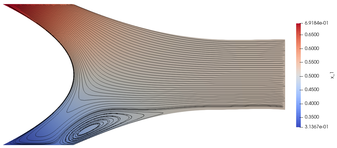
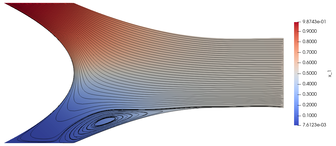
The mole fraction and streamlines of benzene for \(v_1^\text{ref}=0.4\times 10^{-6}\) and \(v_1^\text{ref}=0.4\times 10^{-5}\) are displayed below on the left and right respectively. Owing to parameter continuation and the high-order discretisation, we can robustly solve the problem even in the presence of low species concentrations and sharp solution gradients.
|
|
A Python script version of this demo can be found here.
References
Francis R. A. Aznaran, Patrick E. Farrell, Charles W. Monroe, and Alexander J. Van-Brunt. Finite element methods for multicomponent convection-diffusion. IMA J. Numer. Anal., 45(1):188–222, 2025. doi:10.1093/imanum/drae001.
Aaron Baier-Reinio and Patrick E. Farrell. High-order finite element methods for three-dimensional multicomponent convection-diffusion. SIAM J. Sci. Comput., 48(2):A540–A567, 2026. doi:10.1137/25M1734385.
Don W. Green and Robert H. Perry. Perry’s Chemical Engineers’ Handbook. McGraw Hill Professional, 8th edition, 2007.
Rajamani Krishna and Johannes A Wesselingh. The Maxwell–Stefan approach to mass transfer. Chemical Engineering Science, 52(6):861–911, 1997. doi:10.1016/S0009-2509(96)00458-7.